Diss. ETH Nr. 15652
EARTHQUAKE SOURCE PARAMETERS IN THE
ALPINE-MEDITERRANEAN REGION FROM SURFACE
WAVE ANALYSIS
A dissertation submitted to the
Swiss Federal Institute of Technology
Zürich, Switzerland
Dissertation for the degree of
Doctor of Natural Sciences
presented by
Fabrizio Bernardi
Dipl. Natw. ETH
Born on June 30, 1973
Citizen of Stabio - TI, Switzerland
Accepted on the recommendation of
Prof. Dr. Domenico Giardini, examiner
Dr. Jochen Braunmiller, co-examiner
Dr. Urs Kradolfer, co-examiner
Prof. Dr. Torsten Dahm, co-examiner
2004
_______________________________________________________________________________________
Contents
_______________________________________________________________________________________
Abstract
In this thesis, I present two methods to retrieve earthquake source parameters from regional
surface wave data for moment magnitude Mw > 4.3 earthquakes. The first method involves fast
and fully automatic moment tensor (MT) computation. Automatization includes near real-time
earthquake alert screening, data collection from near-real time accessible broad-band stations at
regional distances ( < 20o), MT computation, solution quality assessment and dissemination.
The routine is triggered by events with magnitude M > 4.7 in the European-Mediterranean
region. MTs are computed using long period data with PREM synthetics. I tested various long
period pass bands to evaluate the influence of location accuracy and of simple 1D
synthetics on MT retrieval. The best fixed period band for the entire region is currently
50 - 100 s, because relatively few stations are near-real time accessible and often
the quickly available locations are of low precision. To assess solution quality, the
automatic results are compared with the independent, manually derived Swiss regional
moment tensor catalog. Solutions are divided into three qualities. Near real-time
application from April 2000 to April 2002 resulted in 38 quality A, with well resolved
Mw, depth and focal mechanism, 21 B, with well resolved Mw and 28 unreliable
quality C solutions. For Mw > 5.5 we consistently obtained A solutions. Between
Mw = 4.5 - 5.5 we obtained quality A and B. In a second step, I significantly improved MT
retrieval relative to the standard routine by selecting different period bands for each
station and component. The band width depends on the epicentral distance and on the
signal-to-noise ratio of each period within each seismogram component. For events in the
eastern Mediterranean Sea and the near East, the shortest period used is 50 s. For
events in Europe, the short period cut-off varies from 35 s for close stations to 50 s for
distant stations. Only periods that exceed a signal-to-noise ratio Rm are actually used.
The use of shorter periods and removal of noisy data leads to an improvement of
solution quality for 4.3 < Mw < 4.7 earthquakes. For events between May 2002 and
September 2003 the new routine provided 20% more quality A solutions than the
standard routine. Successful analysis of more smaller earthquakes with the new routine
suggests to lower the currently implemented trigger magnitude from M > 4.7 to about
M > 4.3.
< 20o), MT computation, solution quality assessment and dissemination.
The routine is triggered by events with magnitude M > 4.7 in the European-Mediterranean
region. MTs are computed using long period data with PREM synthetics. I tested various long
period pass bands to evaluate the influence of location accuracy and of simple 1D
synthetics on MT retrieval. The best fixed period band for the entire region is currently
50 - 100 s, because relatively few stations are near-real time accessible and often
the quickly available locations are of low precision. To assess solution quality, the
automatic results are compared with the independent, manually derived Swiss regional
moment tensor catalog. Solutions are divided into three qualities. Near real-time
application from April 2000 to April 2002 resulted in 38 quality A, with well resolved
Mw, depth and focal mechanism, 21 B, with well resolved Mw and 28 unreliable
quality C solutions. For Mw > 5.5 we consistently obtained A solutions. Between
Mw = 4.5 - 5.5 we obtained quality A and B. In a second step, I significantly improved MT
retrieval relative to the standard routine by selecting different period bands for each
station and component. The band width depends on the epicentral distance and on the
signal-to-noise ratio of each period within each seismogram component. For events in the
eastern Mediterranean Sea and the near East, the shortest period used is 50 s. For
events in Europe, the short period cut-off varies from 35 s for close stations to 50 s for
distant stations. Only periods that exceed a signal-to-noise ratio Rm are actually used.
The use of shorter periods and removal of noisy data leads to an improvement of
solution quality for 4.3 < Mw < 4.7 earthquakes. For events between May 2002 and
September 2003 the new routine provided 20% more quality A solutions than the
standard routine. Successful analysis of more smaller earthquakes with the new routine
suggests to lower the currently implemented trigger magnitude from M > 4.7 to about
M > 4.3.
The second method retrieves seismic moment Mo directly from surface wave amplitudes
recorded at regional distances. The amplitude-moment relation is derived from digital
broad-band data of 18 earthquakes (3.9 < Mw < 5.1) in and near Switzerland with independent
Mo values. The amplitudes were measured at empirically determined, distance varying,
reference periods T . For amplitudes measured at T, the distance attenuation term of the
surface wave magnitude relation S() = log(A/T)max + 1.66log is independent of distance.
Mo is then defined by logMo = S() + 14.90 assuming 1:1 scaling of log Mo - MS, which is
true for MS
. For amplitudes measured at T, the distance attenuation term of the
surface wave magnitude relation S() = log(A/T)max + 1.66log is independent of distance.
Mo is then defined by logMo = S() + 14.90 assuming 1:1 scaling of log Mo - MS, which is
true for MS  7.2 in continental areas. Uncertainties of ±0.30 for the 14.90-constant
correspond to a factor of 2Mo uncertainty, which was verified with independent data. This
relation allows fast, direct Mo determination which can be applied to any earthquake.
Re-calibration of the 14.90-constant, however, is probably required for other tectonic regions.
I applied the amplitude-Mo relation to determine Mo of 25 stronger 20th century
events in Switzerland from analog data. The data recorded by early instrumental
seismographs were collected from several European observatories. Amplitudes were measured
from scans at large magnification and corrected for differences between T and the
actual measurement period. The resulting magnitudes range from Mw = 4.6 to 5.8.
The Mw = 5.8 1946 event in the Valais was the largest 20th century earthquake.
Magnitude uncertainties for the early-instrumental events are on the order of 0.4
units. The Mo estimates were then used for the up-date of the Earthquake Catalog of
Switzerland to calibrate an intensity-Mo relationship for pre-instrumental data. Accurate
intensity-Mo relations are fundamental for improved seismic hazard evaluations in
regions characterized by moderate seismicity and by long recurrence times of larger
events.
7.2 in continental areas. Uncertainties of ±0.30 for the 14.90-constant
correspond to a factor of 2Mo uncertainty, which was verified with independent data. This
relation allows fast, direct Mo determination which can be applied to any earthquake.
Re-calibration of the 14.90-constant, however, is probably required for other tectonic regions.
I applied the amplitude-Mo relation to determine Mo of 25 stronger 20th century
events in Switzerland from analog data. The data recorded by early instrumental
seismographs were collected from several European observatories. Amplitudes were measured
from scans at large magnification and corrected for differences between T and the
actual measurement period. The resulting magnitudes range from Mw = 4.6 to 5.8.
The Mw = 5.8 1946 event in the Valais was the largest 20th century earthquake.
Magnitude uncertainties for the early-instrumental events are on the order of 0.4
units. The Mo estimates were then used for the up-date of the Earthquake Catalog of
Switzerland to calibrate an intensity-Mo relationship for pre-instrumental data. Accurate
intensity-Mo relations are fundamental for improved seismic hazard evaluations in
regions characterized by moderate seismicity and by long recurrence times of larger
events.
_______________________________________________________________________________________
Riassunto
In questo lavoro sono presentati due metodi, i quali, utilizzando onde di superficie, permettono
di determinare i parametri della sorgente di terremoti regionali con magnitudine Mw > 4.3. Il
primo calcola velocemente ed in maniera completamente automatica il tensore momento. Il
processo di automatizzazione include l’analisi delle localizzazioni automatiche provenienti da
diverse agenzie, la richiesta dei dati in tempo reale da stazioni a banda larga situate a distanza
regionale ( < 20o), il calcolo del tensore momento, la deteminazione dell’affidabilita della
soluzione e la sua pubblicazione (sul web e via e-mail). La procedura analizza ogni
evento dichiarato con magnitudine M > 4.7 e localizzato in Europea e nell’ area
mediterranea. I tensori momento sono calcolati usando dati reali a lungo periodo
e librerie di sismogrammi sintetici calcolati con modello PREM. Sono stati testati
diversi intervalli di periodo, focalizzando l’analisi sulla stabilitá delle soluzioni in base
alla precisione della localizzazione usata ed ai sismogrammi sintetici calcolati per un
semplice modello 1D. La bassa affidabilità delle localizzazioni disponibili e l’ancora
scarsa disponibilità di dati a banda larga in tempo reale evidenziano che l’intervallo
compreso tra i 50 ed i 100 secondi risulta essere il più adatto per l’analisi dei terremoti
nell’intera area europea e mediterranea. Il confronto dei risultati con un catalogo
indipendent di soluzioni tensore momento ha permesso di stabilire le regole generali per
determinare l’affidabilità delle soluzioni così ottenute. Quest’ultime sono state quindi
divise in tre gruppi: soluzioni di ’tipo A’, con momento sismico Mo, profondità e
meccanismo focale affidabili; soluzioni di ’tipo B’, con il solo valore di Mo affidabile ed
infine, soluzioni di ’tipo C’, per cui nessuno dei tre parametri elencati può essere
considerato affidabile. Durante il periodo compreso tra l’aprile 2000 e l’aprile 2002, la
procedura ha ottenuto 28 soluzioni di tipo A, 21 di tipo B e 28 di tipo C. Per eventi con
Mw > 5.5 generalmente si sono ottenute soluzioni di tipo A, mentre per eventi con
Mw = 4.5 - 5.5 si sono ottenuti soluzioni di tipo A e B. In seguito la procedura è stata
significativamente migliorata selezionando l’intervallo dei periodi in base alla distanza e al
rapporto tra il segnale ed il rumore contenuto nei sismogrammi. Pertanto, eventi nel
Mediterraneo orientale e nel vicino oriente sono stati analizzati con periodi compresi
tra 50 e 100 secondi, mentre, quelli verificatisi in Europa, con il periodo più corto
che varia tra i 35 s per le stazioni più vicine ed i 50 s per quelle più lontane. Inoltre
sono stati utilizzati solo i periodi il cui segnale supera un determinato rapporto tra
segnale e rumore, Rm. L’utilizzo di periodi più corti e la rimozione di sismogrammi
contenenti rumore permettono un significativo miglioramento soprattutto per eventi
con magnitudine 4.3 < Mw < 4.7. L’analisi di eventi occorsi tra il maggio 2002 ed
il settembre 2003 con la nuova procedura ha prodotto 66 soluzioni con qualità A,
migliorando del 20% le prestazioni rispetto alla prima procedura. L’efficacia della
nuova procedura suggerisce di spostare la magnitudine di soglia da M > 4.7 verso
M > 4.3.
Con il secondo metodo è possibile calcolare il momento sismico Mo direttamente
dall’ampiezza delle onde di superficie. La relazione tra l’ampiezza ed il momento sismico è stata
derivata utilizzando dati digitali di 18 terremoti (3.9 < Mw < 5.1) occorsi recentemente in
Svizzera e nelle zone limitrofe, per i quali esistono stime indipendenti del momento sismico
ottenute tramite inversione del tensore momento. L’ampiezza delle onde di superficie à
stata misurata con periodi di riferimento T dipendenti dalla distanza e determinati
empiricamente, cosicché il termine dell’attenuazione della magnitudine delle onde di superficie
S() = log(A/T)max + 1.66log non varia più rispetto alla distanza tra stazione ed evento.
Assumendo un rapporto di 1:1 per l’espressione log Mo - MS, considerata valida per terremoti
continentali con magnitudine MS 7.2, il momento sismico è di conseguenza definito
dalla relazione logMo = S() + 14.90. L’incertezza di ±0.30 della costante 14.90
porta ad un fattore di incertezza di 2Mo, verificato con dati indipendenti. Questa
relazione permette di ottenere velocemente una stima di Mo per terremoti recenti
ed è applicabile in ogni regione dopo aver ricalibrato la costante. L’applicazione a
sismogrammi registrati su strumenti meccanici ed elettromeccanici, raccolti in vari osservatori
europei ha permesso di determinare il momento sismico di 25 terremoti verificatisi
in Svizzera e nelle zone limitrofe durante il 20o secolo. Attraverso l’ingrandimento
digitale delle immagini dei sismogrammi si è potuta effettuare una precisa lettura
dell’ampiezza e del periodo. Questo è stato successivamente corretto rispetto il periodo di
riferimento T. Le magnitudini Mw ottenute risultano comprese tra 4.6 e 5.8, quest’ultima
per il più forte terremoto avvenuto in Svizzera (1946, Vallese). L’incertezza della
magnitudine determinata con questi strumenti è di circa 0.4. I valori di Mo ottenuti
hanno permesso la calibrazione tra l’intensità ed il momento sismico per gli eventi
pre-strumentali, utile all’aggiornamento del catalogo dei terremoti in Svizzera (ECOS). Precise
relazioni tra in momento sismico e l’intensità sono fondamentali per ottenere stime
affidabili del l’azzardo sismico in regioni a sismicità moderata e con lunghi tempi di
ricorrenza.
Chapter 1
Introduction
In this thesis I present two methods to retrieve earthquakes source parameters (seismic moment
Mo, depth and focal mechanism) for moderate to strong earthquakes from regional surface
waves. The first method, described in chapters 3 and 4, performs fully automatic
and near-real time waveform inversion for the seismic moment tensor. The primary
motivation is to provide rapid magnitude and depth estimates after strong and potentially
damaging events to assist disaster relief agencies’ response efforts. The second method,
described in chapter 5, retrieves Mo from surface wave amplitudes and can be applied to
digital broad band seismograms or to early-instrumental analog seismograms. Here,
this method is applied to derive Mo from 20th century analog data, that are crucial
for long term seismic hazard studies in areas characterized by low and moderate
seismicity.
Fast intervention of disaster relief agencies needs accurate Mo and depth estimates within a
short time after a potentially destructive event. In the European-Mediterranean area seismicity
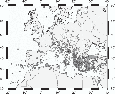
is mainly located in the eastern Mediterranean Sea (Figure 1.1), where several destructive
earthquakes (e.g. the Mw = 7.6 August 17, 1999 Izmit event) occurred during the last years. In
Europe and in the central and western Mediterranean Sea seismicity is lower, but strong
destructive earthquakes are not rare (e.g. the Mw = 6.0 September 6, 2002 Molise,
the Mw = 7.0 May 21, 2003 Northern Algeria and the Mw = 6.4 February 24, 2004
Morocco earthquakes). When such an earthquake occurs, tele-communications in and
around the epicentral area are often interrupted. Magnitude and depth estimates,
that are crucial for damage evaluation, can then be estimated only using far-field
seismological data. Moment tensor (MT) analysis is particularly well suited because MT
inversion prevents underestimation of the magnitude compared to the standard location
techniques, since moment tensor derived seismic moment of large events does not saturate
(Kanamori, 1977).
Fast size and depth estimates are also important after moderate events that do not cause
serious damages, but are widely felt. Thanks to the world-wide-web, people search for
information immediately after a felt earthquake. In Europe even after a moderate event, a large
number of people want to be quickly informed about its magnitude and its consequences.
For this reason the press, police and civil protection agencies need fast and precise
information about location, size and depth of the earthquake. An example is the recent
Mw = 4.5 February 23, 2004 Rigney eastern France event, that was felt over the
western part of Switzerland. Within minutes the Swiss Seismological Service got
swamped with calls from concerned people and press, and the web-server was heavily
accessed.
Quick moment tensor solutions are routinely provided by several groups at a global scale but
only for large events (Mw > 5.5). These solutions are disseminated only after revision
by a seismologist. Moment tensor solutions for moderate (Mw > 4.8) events in the
European-Mediterranean region are now provided by the Swiss Seismological Service, the Italian
INGV and the Spanish IGN. Such solutions are computed manually and only for the more
relevant earthquakes the moment tensor is available within hours after event origin time, while
other earthquakes are analyzed with a delay of weeks to months. The routine presented here
computes fully automatic moment tensors from earthquake alert detection, to data collection,
moment tensor inversion, solution assessment and finally solution dissemination (via
e-mail and web). Computing fully automatic, near-real time moment tensors for a
moderate event (4.5 < Mw < 5.0) requires near-real time access to dense networks of
broadband and high dynamic range seismometer at regional distance ( < 20o). Significant
technological improvements and infrastructure investments during the last few years in the
European-Mediterranean area allowed the development and implementation of the procedure
described here.
The seismic moment tensor provides not only size and depth estimates to alert disaster
relief agencies. Earthquake focal mechanisms, that can be obtained from the seismic
moment tensor, provides indispensable information for seismotectonic studies, e.g. for
stress field estimation in Switzerland (Kastrup et al., 2004). The strain rate tensor,
that can be computed from the moment tensor, combined with GPS measurements
and geological data can then be used to infer deformation fields of the crust, e.g. for
deformation fields in the eastern Mediterranean See (Jenny et al., 2004). Seismic
hazard studies then need accurate magnitude and depth estimates. The automatic
routine presented here, will over time result in a complete moment tensor catalog that
includes also moderate events, which are significant for regions of low and moderate
seismicity.
The Swiss Seismological Service evaluates the seismic hazard in Switzerland. Accurate
seismic hazard maps are indispensable for defining building codes in densely populated and
industrialized regions or nuclear power plant construction requirements. An example is the
Basel area, where strong destructive earthquakes have occurred in the past (e.g. the Mw = 6.9
1356 event, which is the largest event known in Europe north of the Alps) and where numerous
chemical plants are operating. To evaluate seismic hazard for such areas with long
term recurrent seismicity, requires a complete earthquake catalog covering long time
periods.
The Swiss Seismological Service recently completed a comprehensive up-date of the
earthquake catalog of Switzerland and surrounding regions (Fäh et al., 2003). The catalog
expresses the size of all events using moment magnitude (Mw). The largest part of the catalog
includes pre-instrumental events where only epicentral intensities are available. For
these events, the epicentral intensities were linked to the seismic moment using a
epicentral intensity - seismic moment relation that was inferred using earthquakes with
both epicentral intensity and seismic moment available. To enlarge this data-set, also
the major 20th century events that occurred within or near Switzerland were used.
Seismic moment determination of these events constitutes the second large part of this
thesis.
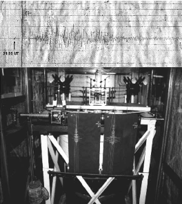
For these events, I collected analog seismograms from various observatories in Europe that
were recorded on mechanical and electromagnetic seismographs for which the instrument
response is well known and the instrument calibrations were available. Figure 1.2 shows an
example of a Wiechert seismograph and one of its recordings. Because of the low quality of such
records, a reliable digitization was not possible for most of the collected data-set and, thus, the
moment tensor inversion technique could not be applied to derive Mo estimates for most of the
events investigated. Nevertheless, accurate readings of amplitude and periods were possible. I
thus developed a method to evaluate seismic moment (Mo) directly from surface wave
amplitude. The method, developed using broad-band digital seismograms of recent events, was
then applied to the early-instrumental seismograms of the 20th century major Swiss
events.
Chapter 2
Brief overview of seismic moment tensor
The seismic moment tensor describes
the earthquake source as a point source. The earthquake source parameters like focal
mechanism (strike, dip, slip) and magnitude (seismic moment Mo) follow from the moment
tensor. The displacement u(x,t) can be written as (Aki & Richards, 2002)
![integral oo integral integral
-d--
un(x, t) = - oo dt S[ui(q,t )]cijpqnjdqq Gnp(x, t- t;q, 0)dS](main2x.gif) | (2.1) |
where Gnp(x,t -  ;
;  , 0) is the n-th component of the earth at the station in response to a
unit-force excitation in p-direction at the source (Green function). is a general position on the
fault surface
, 0) is the n-th component of the earth at the station in response to a
unit-force excitation in p-direction at the source (Green function). is a general position on the
fault surface  and x is the station. Using the convolution, equation 2.1 can be rewritten
as
and x is the station. Using the convolution, equation 2.1 can be rewritten
as
![integral integral
d
un(x,t) = [ui]cijpqnj * dqqGnpdS
S](main3x.gif) | (2.2) |
Equation 2.2 refers to a displacement un(x,t) caused by a dislocation along a fault plane
of finite extent. Assuming that the periods considered are much longer than the source volume,
the earthquake source can be approximated by a point source, reducing equation 2.2
is
 | (2.3) |
where Mpq = 
 [ui]
[ui] jcijpq is the seismic moment tensor. Knowing u(x,t) (measured at
seismic stations) and Gnq,p(x,t) (computed for any Earth), the MT is then computed
solving
jcijpq is the seismic moment tensor. Knowing u(x,t) (measured at
seismic stations) and Gnq,p(x,t) (computed for any Earth), the MT is then computed
solving
 | (2.4) |
The method used in this thesis to solve for the MT uses amplitude spectra of observed and
synthetic seismograms (Giardini, 1992). Using amplitude spectra avoids artifacts
caused by filters used to select the inverting period band, that are generally used for
inversion techniques in the time domain, and allows to select different period bands
for different stations and components maintaining a linear approach to solve the
moment tensor. This approach allows a significant improvement of the results for
small and moderate events when only a sparse seismic network is available (chapter
4).
A moment tensor can be decomposed into elementary tensors following two different
approaches: a pure mathematical decomposition or a decomposition into source components
with a physical meaning (e.g. double-couple, explosion, tension crack components,
etc.). The decomposition into physical sources is not unique. The paper of Jost &
Herrmann (1989) gives an excellent overview on the different decomposition methods that are
generally applied in seismology. The MT decomposition performed in this thesis is
described in the next paragraphs. Generally the MT can be decomposed uniquely
into an isotropic and a deviatoric part. In order to derive a general formulation of
the moment tensor decomposition, let mi be the eigenvalues corresponding to the
orthogonal eigenvector ai = (aix,aiy,aiz)T of M
pq. Using the orthogonality of the
eigenvectors, we can write the principal axis transformation of M in reverse order
as:
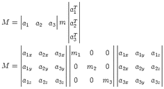 | (2.5) |
From equation 2.5, we find relations between components of the eigenvectors and the
moment tensor elements:
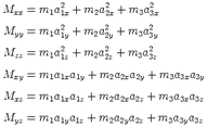 | (2.6) |
where m in equation 2.5 is the diagonalized moment tensor and the elements of m are the
eigenvalues of M. The general moment tensor decomposition can now be defined by rewriting m
as:
 | (2.7) |
where tr(M) = m1 + m2 + m3 is the trace of the moment tensor and mi* are purely
deviatoric eigenvalues mi - tr(M). The first term of equation 2.7 describes the isotropic part
of the diagonalized moment tensor, and is important to quantify the volume change in the
source. The second term describes the deviatoric part and can be further decomposed using
different approaches.
tr(M). The first term of equation 2.7 describes the isotropic part
of the diagonalized moment tensor, and is important to quantify the volume change in the
source. The second term describes the deviatoric part and can be further decomposed using
different approaches.
In this study the deviatoric part is decomposed into a double-couple component and a
compensated linear vector dipole (CLVD) (Knopoff & Randall, 1970). Assuming
|m3*|<|m
2*|<|m
1*| the deviatoric part can be rewritten as
 | (2.8) |
where F = -m1*/m
3* and (F - 1) = m
2*/m
3*. Note that 0 < F < 0.5. Equation 2.8 can
then be decomposed into two parts representing a double couple and a CLVD
 | (2.9) |
Such decomposition has the advantage that both double couple and CLVD components have
the same orientation of their principal axis system (chapter 3). To estimate the deviation of the
seismic source from the model of a pure double couple Dziewonski et al. (1981) used the
parameter
 | (2.10) |
For a pure double couple  = 0 (mmin* = 0), while for a pure CLVD mechanism
= 0.5.
= 0 (mmin* = 0), while for a pure CLVD mechanism
= 0.5.
The focal mechanism (strike, dip and slip) of the earthquake can be solved from the six
elements of the seismic moment tensor:
 | (2.11) |
where  is the dip,
  the slip and
  the strike.
The magnitude of an earthquake can be expressed in term of scalar seismic moment Mo
that can be determined from the seismic moment tensor:
 | (2.12) |
where m1 and m2 are the largest eigenvalues in absolute sense. The moment magnitude Mw
is defined as (Kanamori, 1977):
 | (2.13) |
The depth of the earthquake centroid (same as hypocenter for small earthquakes) is
retrieved by multiple trials of the moment tensor inversions for different depths. We
do not invert for the centroid location. For each solution we obtain the normalized
variance
 | (2.14) |
The best hypocenter depth is assumed to be at the depth with the smallest normalized
variance.
A more extensive and detailed description of the seismic moment tensor can be found in Jost
& Herrmann (1989), Dahlen & Tromp (1998) and in Aki & Richards (2002). For details of the
MT code see Giardini (1992).
Chapter 3
Automatic regional moment tensor inversion in the European-Mediterranean
region
3.1 Summary
We produce fast and automatic moment tensor solutions for all moderate to strong earthquakes
in the European-Mediterranean region. The procedure automatically screens near real-time
earthquake alerts provided by a large number of agencies. Each event with magnitude
M > 4.7 triggers an automatic request for near real-time data at several national and
international data centers. Moment tensor inversion is performed using complete
regional long period (50 - 100 s) waveforms. Initially the data are inverted for a fixed
depth to remove traces with a low signal-to-noise ratio. The remaining data are then
inverted for several trial depths to find the best-fit depth. Solutions are produced within
90 minutes after an earthquake. We analyze the results for the April 2000 to April
2002 period to evaluate the performance of the procedure. For quality assessment, we
compared the results with the independent Swiss regional moment tensor catalog
(SRMT) and divided the 87 moment tensor solutions into three groups: 38 quality A
with well-resolved Mw, depth and focal mechanism; 21 quality B with well-resolved
Mw; and 28 unreliable quality C solutions. The non-homogeneous station and event
distribution, varying noise level, and inaccurate earthquake locations affected solution
quality. For larger events (Mw > 5.5) we consistently obtained quality A solutions.
Between Mw = 4.5 - 5.5 we obtained quality A and B solutions. Solutions that pass
empirical rules mimicking the a posteriori quality for our data set are automatically
disseminated.
3.2 Introduction
Quick and accurate source parameter determination (magnitude, depth and focal mechanism)
provides important information for fast intervention in areas strongly damaged by large
earthquakes. When compared to standard determination of earthquake location and magnitude,
moment tensor inversion usually provides more accurate source parameters and particularly
so for the size of large events, since their moment magnitudes Mw do not saturate
(Kanamori, 1977). The recent increase in the number of near real-time accessible broadband
stations in the European-Mediterranean region now allows automatic, near real-time moment
tensor analysis monitoring strong events.
Accurate and quick moment tensor inversion is routinely performed on a global scale by the
Harvard Centroid-Moment Tensor (CMT) project (Dziewonski et al., 1981; Dziewonski &
Woodhouse, 1983), the United States Geological Survey (Sipkin, 1982, 1986) and the
Earthquake Research Institute (ERI), Japan (Kawakatsu, 1995). These approaches use
teleseismic data, limiting analysis to stronger earthquakes (Mw > 5.5). Analysis of smaller
earthquakes requires data recorded at regional distances, which is becoming possible with the
growing number of broadband seismic networks. Several groups in the United States (Dreger &
Helmberger, 1993; Ritsema & Lay, 1993; Romanowicz et al., 1993; Náb lek &
Xia, 1995; Braunmiller et al., 1995; Thio & Kanamori, 1995; Dreger et al., 1995; Pasyanos
et al., 1996) and Japan (Kubo et al., 2002), routinely invert for the seismic moment tensor
using seismic data recorded at near regional distances ( < 10o).
lek &
Xia, 1995; Braunmiller et al., 1995; Thio & Kanamori, 1995; Dreger et al., 1995; Pasyanos
et al., 1996) and Japan (Kubo et al., 2002), routinely invert for the seismic moment tensor
using seismic data recorded at near regional distances ( < 10o).
In the European-Mediterranean region, event-station distances are generally larger
( > 10o) than in the western United States. However, several studies (Arvidsson &
Ekstrom, 1998; Braunmiller, 1998) showed that source parameters of moderate events can be
determined routinely with long period regional data (T > 30 - 40s) for larger event-station
distances. The Swiss Seismological Service (Braunmiller et al., 2000, 2002) and the Italian
Istituto Nazionale di Geofisica e Vulcanologia (INGV) (Pondrelli et al., 2002) now routinely
produce moment tensor solutions in the European-Mediterranean area for moderate to strong
earthquakes (Mw > 4.5), and smaller earthquakes (Mw > 3.0) in the Alpine area (Braunmiller
et al., 2000, 2002). Small to moderate earthquakes in the western Mediterranean
region are regularly processed by the Spanish Instituto Andaluz de Geofísica (Stich
et al., 2003).
Here we test whether the current near real-time data availability and location accuracy are
sufficient for automatic regional moment tensor retrieval using intermediate to long period
surface waves (50 - 100 s). Our goal is to develop a robust procedure that provides
fully automatic, fast and reliable solutions for moderate to strong earthquakes in the
European-Mediterranean region.
Our automatic procedure consists of two main parts: first, moment tensor inversion for a
detected earthquake and second, automatic quality assessment of the solution. We first
describe the method and show the reliability of the automatic solutions. Then we
present empirical rules for automatic quality assessment. Finally, we discuss source
parameters (focal mechanism, depth and Mw) and investigate factors that affect solution
quality.
3.3 Data and method
Ultimately, we like to obtain a moment tensor within a few minutes after an event.
This requires on-line data access to stations at close epicentral distances, currently
unavailable for most of our study region. We anticipate that present waiting periods due to
sparse networks and time delays for data acquisition will shorten considerably in the
future.
3.3.1 Data acquisition
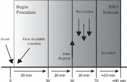
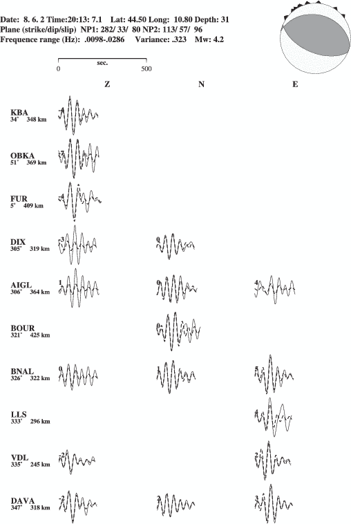
Automatic moment tensor inversion consists of several steps (Figure 3.1). A few minutes after
an event, an automatic earthquake alert (location, magnitude) is generally available, provided
by the Swiss Seismological Service (SED) and other agencies linked to our institute. Automatic
information coming from many agencies may include false alarms, but guarantees
that we miss no significant event. We screen incoming information and any event
in the European-Mediterranean area (22o < Lat < 68o,-25o < Long < 60o) with
magnitude M > 4.7, independent of magnitude type [ML,mb,MS], starts the routine
automatically.
We invert complete broadband waveforms recorded at regional epicentral distances
( < 20o); therefore, our data window is 30 minutes long. We wait an additional 20 minutes to
assure data availability (Figure 3.1) before sending data requests to the AutoDRM
(Kradolfer, 1996) of several international (ORFEUS, USGS) and national data centers (in
Austria, Czech Republic, Germany, Israel, Norway, Switzerland) that provide near real-time
broadband seismograms. The data centers automatically process these requests and usually
within 20 minutes all available seismograms are received at our server to be stored and prepared
for inversion. 70 minutes after event origin time, data acquisition is considered complete and the
inversion starts, resulting in an automatic moment tensor solution within 90 minutes after an
earthquake.
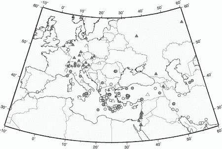
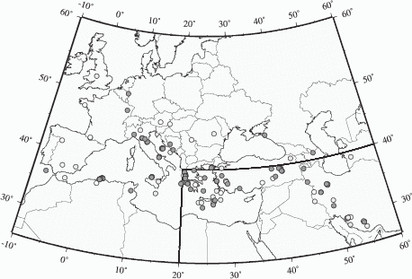
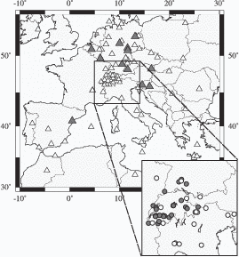
Between April 2000 and April 2002 only stations in central and northern Europe, Israel, the
Caucasus region and Russia provided near real-time data (black triangles in Figure 3.2). Data
availability and the response time of data centers varied. To ensure that we received a sufficient
number of seismograms, we chose a relatively long waiting period before requesting
data and starting the inversion. Stations in the western and central Mediterranean
Sea, Turkey and eastern Europe (white triangles in Figure 3.2), became available
during mid-2002 and are only shown to illustrate the evolving and improving station
coverage.
3.3.2 Algorithm
The algorithm uses intermediate to long period three-component regional data. The inversion
code, described in Giardini (1992), has already been applied to many earthquakes
(Giardini, 1992; Giardini et al., 1993a,b; Sicilia, 1999). Synthetic seismograms are generated
by normal mode summation (Woodhouse, 1988) computed for the PREM-Earth model
(Dziewonski & Anderson, 1981) at different source depths and stored in libraries for quick
access. The moment tensor is constrained to be deviatoric. We do not invert for the source
centroid but compute time corrections by re-aligning data and synthetics (Giardini, 1992).
Depth is retrieved by minimizing the normalized variance (defined as ratio of variance over data
vector norm) for different trial depths.
3.3.3 Inversion
The moment tensor inversion automatically starts 70 minutes after an event (Figure 3.1). The
alert is the first available location, which is not necessarily the best epicenter estimate. 70
minutes after an event, several automatic and/or manual locations are usually available and we
choose the a priori most accurate. We prefer a location from a network that surrounds the
epicenter. When that is not available, we look for a manual location or one provided by an
agency with a large aperture network.
The seismograms are bandpass filtered between 50 and 100 s period. A lowpass filter at 50 s
applied to regional seismograms minimizes the effect of inaccurately known propagation paths
and allows moment tensor retrieval of moderate sized earthquakes (Mw > 4.5) with a simple
average 1D velocity model (Arvidsson & Ekstrom, 1998). We tested other filter parameters and
report results in Section 3.5.2.
The automatic inversion consists of two main steps. First, the entire data set is inverted for
a fixed depth (18 km) to remove traces with a low signal-to-noise ratio (high normalized
variance > 0.8) and large re-alignment. From tests we found, that the choice of the fixed depth -
18 km or different depth - has little effect on the remaining data set and basically no effect on
our results. The remaining traces are then inverted for several depths. The 50 - 100 s data have
little depth resolution, because long period surface-wave excitation functions have little depth
variation. Thus, we apply a limited number of depth-steps with increasing step width
(10, 14, 18, 25, 31, 42, 55, 75, 100, 125, 150, 175 and 200 km) to find the best fitting
depth. We use a minimum 10% variance increase to estimate depth uncertainty; our
uncertainty range is simply defined by the trial depths that just exceed the 10% increase.
We consider this uncertainty estimate conservative, since the waveform fit degrades
visibly.
3.4 Quality assessment of results
We started our procedure for automatic moment tensor inversion in April 2000. By
April 2002, we obtained 87 moment tensor solutions (Figure 3.2, Table 3.1), mainly
for events in the seismically active central-eastern Mediterranean region (Jackson &
McKenzie, 1988).
We check the quality of the automatic moment tensors because solution accuracy depends
on event location, location precision, station distribution and signal strength. First, we use an
independent high-quality moment tensor catalog to quantify true quality. Second, to
estimate solution quality automatically, we derive rules from solution parameters which
reproduce overall true quality. These rules are applied automatically before disseminating
solutions.
3.4.1 True quality
The Swiss automatic moment tensor (SAMT) catalog contains many moderate events not
included in global catalogs, incomplete below Mw = 5.5 and with very few Mw < 5.0 events.
Therefore, we compared our automatic solutions with those of the Swiss Seismological Service’s
regional moment tensor (SRMT) catalog. The SRMT covers the European-Mediterranean area
and is nearly complete down to mb = 4.5 (Braunmiller et al., 2002). SRMT solutions are
derived with a more complete data set available weeks to months after an event than the data
set used for SAMT analysis. SRMT solution quality is high based on comparison with other
independent source parameter estimates available for selected events (Braunmiller
et al., 2002). For a few events east of SRMT coverage (> 55oE), we compared our
solutions with the Harvard catalog, or when not available, with magnitudes given by the
USGS.
| Table 3.1: | Table of the 87 automatic moment tensor solutions. From left to right: Event number, PDE-location, true and
assigned quality, seismic moment Mo in Nm, Mw, depth in km, orientation of the two nodal planes in degree, number of
stations and components used, quickly available location used for inversion. For completeness, we include all source parameters
even for true quality B and C solutions. For B, only size is well resolved and for C, none of the parameters is reliably resolved.
For further studies, use Mw, depth and focal mechanism from A and only Mw from B solutions. |
|
|
|
|
|
|
|
|
|
|
|
|
|
|
|
|
|
|
|
|
|
|
|
| | Nr. | | Location (PDE) Quality | Mo | Mw | Depth | Plane 1 | Plane 2 | St. | Co. | Location used for inversion
|
|
|
|
|
|
|
|
|
|
|
|
|
|
|
|
|
|
|
|
|
|
|
|
| | | Date | Time | Lat | Long | True | Assigned | | | | Strike | Dip | Rake | Strike | Dip | Rake | | | Time | Lat | Long |
|
|
|
|
|
|
|
|
|
|
|
|
|
|
|
|
|
|
|
|
|
|
|
| | 1 | 00-04-06 | 00:10:38.0 | 45.72 | 26.58 | A | Aa | .410E+17 | 5.01 | 125 | 0 | 20 | 58 | 213 | 72 | 101 | 27 | 50 | 00:10:39.0 | 45.70 | 26.60 |
| 2 | 00-04-21 | 12:23:10.0 | 37.83 | 29.31 | B | Ba | .114E+18 | 5.31 | 31 | 336 | 49 | -48 | 103 | 55 | -127 | 11 | 13 | 12:23:05.0 | 36.80 | 29.40 |
| 3 | 00-05-24 | 05:40:37.7 | 36.04 | 22.01 | A | Aa | .528E+18 | 5.75 | 25 | 269 | 47 | 4 | 176 | 86 | 137 | 20 | 44 | 05:40:35.7 | 36.10 | 21.90 |
| 4 | 00-06-06 | 02:41:49.8 | 40.69 | 32.99 | A | Aa | .128E+19 | 6.01 | 10 | 8 | 43 | -31 | 122 | 68 | -128 | 26 | 66 | 02:41:56.7 | 41.30 | 32.90 |
| 5 | 00-06-13 | 01:43:14.0 | 35.15 | 27.13 | A | Aa | .126E+18 | 5.34 | 18 | 227 | 82 | 1 | 137 | 88 | 172 | 28 | 74 | 01:43:18.0 | 35.30 | 27.20 |
| 6 | 00-06-15 | 21:30:29.0 | 34.44 | 20.18 | A | Ba | .352E+17 | 4.97 | 42 | 40 | 45 | 65 | 253 | 49 | 112 | 10 | 16 | 21:30:34.4 | 34.50 | 20.00 |
| 7 | 00-07-25 | 19:33:56.0 | 37.13 | 21.99 | A | Aa | .442E+17 | 5.03 | 42 | 333 | 36 | -62 | 119 | 57 | -109 | 25 | 41 | 19:33:47.7 | 37.50 | 24.00 |
| 8 | 00-08-21 | 17:14:26.0 | 44.87 | 8.48 | A | Aa | .281E+17 | 4.90 | 10 | 114 | 34 | -113 | 322 | 59 | -74 | 30 | 65 | 17:14:26.0 | 44.80 | 8.60 |
| 9 | 00-08-23 | 13:41:28.0 | 40.68 | 30.72 | A | Aa | .187E+18 | 5.45 | 31 | 251 | 71 | -168 | 157 | 78 | -18 | 29 | 77 | 13:41:26.0 | 40.40 | 30.70 |
| 10 | 00-11-15 | 15:05:37.0 | 38.35 | 42.93 | A | Aa | .288E+18 | 5.58 | 18 | 217 | 20 | 37 | 92 | 77 | 106 | 5 | 10 | 15:05:24.7 | 38.40 | 44.00 |
| 11 | 00-12-06 | 17:11:06.4 | 39.57 | 54.80 | A | Aa | .307E+20 | 6.93 | 42 | 110 | 44 | 80 | 302 | 46 | 98 | 6 | 18 | 17:11:07.9 | 39.70 | 54.90 |
| 12 | 00-12-15 | 16:44:47.6 | 38.45 | 31.35 | A | Aa | .193E+19 | 6.13 | 18 | 290 | 30 | -96 | 117 | 59 | -86 | 25 | 62 | 16:44:45.0 | 38.60 | 31.10 |
| 13 | 01-02-25 | 18:34:42.2 | 43.46 | 7.47 | A | Aa | .997E+16 | 4.60 | 31 | 249 | 22 | 93 | 65 | 67 | 88 | 16 | 24 | 18:34:32.6 | 42.90 | 7.40 |
| 14 | 01-03-10 | 11:20:57.8 | 35.08 | 26.37 | C | Ba | .640E+17 | 5.14 | 75 | 146 | 46 | 110 | 297 | 47 | 69 | 11 | 23 | 11:20:59.3 | 35.60 | 27.00 |
| 15 | 01-03-23 | 05:24:12.2 | 32.92 | 46.65 | B | Ca | .274E+18 | 5.56 | 18 | 307 | 16 | 22 | 196 | 84 | 104 | 3 | 6 | 05:24:21.8 | 33.60 | 45.30 |
| 16 | 01-03-28 | 16:34:21.8 | 29.69 | 51.18 | C | Ca | .205E+17 | 4.81 | 18 | 313 | 43 | 54 | 178 | 55 | 119 | 5 | 5 | 16:34:22.0 | 29.80 | 51.20 |
| 17 | 01-03-30 | 15:30:49.0 | 38.01 | 30.94 | A | Aa | .115E+17 | 4.64 | 25 | 44 | 29 | -103 | 239 | 61 | -82 | 15 | 24 | 15:30:53.0 | 38.70 | 30.80 |
| 18 | 01-04-03 | 17:36:34.1 | 32.45 | 47.99 | C | Ca | .400E+17 | 5.01 | 18 | 106 | 38 | -139 | 342 | 66 | -59 | 4 | 6 | 17:37:27.0 | 31.50 | 49.80 |
| 19 | 01-04-08 | 06:12:27.8 | 38.38 | 22.18 | B | Ba | .152E+17 | 4.73 | 175 | 337 | 41 | 74 | 177 | 50 | 103 | 15 | 18 | 06:12:27.0 | 38.30 | 22.30 |
| 20 | 01-04-09 | 17:38:39.2 | 40.11 | 20.37 | A | Aa | .307E+17 | 4.93 | 31 | 294 | 68 | 22 | 195 | 69 | 156 | 18 | 35 | 17:38:51.0 | 39.80 | 20.40 |
| 21 | 01-04-10 | 14:00:07.6 | 34.30 | 26.17 | B | Ba | .214E+17 | 4.82 | 42 | 4 | 46 | -164 | 263 | 78 | -44 | 12 | 14 | 14:00:11.0 | 34.30 | 26.10 |
| 22 | 01-05-01 | 06:00:54.1 | 35.64 | 27.49 | A | Ba | .684E+17 | 5.16 | 10 | 337 | 37 | -126 | 199 | 60 | -65 | 12 | 35 | 06:00:55.0 | 35.80 | 27.40 |
| 23 | 01-05-04 | 19:52:01.9 | 34.72 | 22.74 | B | Ca | .272E+17 | 4.89 | 10 | 13 | 25 | 28 | 256 | 78 | 112 | 2 | 3 | 19:52:32.0 | 36.00 | 21.00 |
| 24 | 01-05-17 | 11:43:58.2 | 39.02 | 15.47 | A | Aa | .359E+17 | 4.97 | 200 | 152 | 16 | -149 | 33 | 81 | -75 | 11 | 17 | 11:43:57.5 | 38.90 | 15.50 |
| 25 | 01-05-24 | 17:34:01.1 | 45.75 | 26.46 | A | Aa | .741E+17 | 5.18 | 150 | 0 | 30 | 61 | 212 | 63 | 105 | 22 | 42 | 17:33:55.6 | 45.80 | 26.70 |
|
|
|
|
|
|
|
|
|
|
|
|
|
|
|
|
|
|
|
|
|
|
|
| | |
|
|
|
|
|
|
|
|
|
|
|
|
|
|
|
|
|
|
|
|
|
|
|
|
| | Nr. | | Location (PDE) Quality | Mo | Mw | Depth | Plane 1 | Plane 2 | St. | Co. | Location used for inversion
|
|
|
|
|
|
|
|
|
|
|
|
|
|
|
|
|
|
|
|
|
|
|
|
| | | Date | Time | Lat | Long | True | Assigned | | | | Strike | Dip | Rake | Strike | Dip | Rake | | | Time | Lat | Long |
|
|
|
|
|
|
|
|
|
|
|
|
|
|
|
|
|
|
|
|
|
|
|
| | 26 | 01-05-29 | 04:43:56.4 | 35.39 | 27.75 | A | Ba | .655E+17 | 5.15 | 25 | 314 | 65 | -179 | 224 | 89 | -24 | 12 | 27 | 04:43:56.0 | 35.40 | 27.70 |
| 27 | 01-06-10 | 01:52:08.0 | 39.87 | 55.89 | A | Ca | .132E+18 | 5.35 | 25 | 114 | 34 | 57 | 331 | 61 | 110 | 2 | 2 | 01:52:11.8 | 40.50 | 53.60 |
| 28 | 01-06-22 | 11:54:48.5 | 39.35 | 27.34 | A | Aa | .983E+17 | 5.27 | 25 | 353 | 52 | -17 | 94 | 76 | -141 | 15 | 28 | 11:54:48.0 | 39.40 | 27.70 |
| 29 | 01-06-23 | 06:52:41.9 | 35.71 | 28.02 | B | Ba | .558E+18 | 5.77 | 31 | 239 | 53 | -24 | 345 | 70 | -140 | 10 | 23 | 06:52:45.4 | 35.80 | 28.10 |
| 30 | 01-06-25 | 13:28:46.4 | 37.20 | 36.17 | A | Aa | .199E+18 | 5.47 | 10 | 346 | 19 | -131 | 210 | 75 | -76 | 10 | 25 | 13:28:49.8 | 37.10 | 35.90 |
| 31 | 01-07-10 | 21:42:06.4 | 39.88 | 41.59 | B | Ca | .994E+17 | 5.27 | 31 | 284 | 71 | -170 | 191 | 81 | -18 | 4 | 6 | 21:41:49.9 | 39.20 | 44.30 |
| 32 | 01-07-17 | 15:06:15.6 | 46.74 | 11.37 | A | Aa | .156E+17 | 4.73 | 10 | 208 | 40 | -5 | 302 | 86 | -130 | 10 | 16 | 15:06:16.3 | 47.00 | 11.50 |
| 33 | 01-07-20 | 05:09:39.2 | 45.77 | 26.78 | A | Aa | .433E+17 | 5.03 | 100 | 281 | 12 | 20 | 171 | 85 | 101 | 10 | 25 | 05:09:10.0 | 44.00 | 29.00 |
| 34 | 01-07-26 | 00:21:37.0 | 39.06 | 24.34 | A | Aa | .851E+19 | 6.56 | 25 | 231 | 67 | -178 | 140 | 88 | -22 | 24 | 70 | 00:21:37.5 | 39.10 | 24.30 |
| 35 | 01-07-26 | 04:53:34.0 | 39.02 | 24.28 | A | Aa | .267E+17 | 4.89 | 31 | 243 | 58 | 176 | 335 | 87 | 31 | 13 | 21 | 04:53:33.1 | 39.10 | 24.30 |
| 36 | 01-07-30 | 15:24:57.0 | 39.04 | 24.01 | A | Aa | .478E+17 | 5.06 | 18 | 227 | 64 | -177 | 136 | 88 | -25 | 23 | 56 | 15:25:06.0 | 39.70 | 23.90 |
| 37 | 01-08-22 | 15:58:01.2 | 47.24 | 70.04 | A | Aa | .932E+17 | 5.25 | 18 | 149 | 57 | 172 | 243 | 83 | 32 | 3 | 9 | 15:58:10.1 | 47.70 | 69.30 |
| 38 | 01-09-13 | 15:42:52.2 | 35.54 | 25.97 | B | Ba | .146E+17 | 4.71 | 42 | 227 | 44 | -7 | 322 | 84 | -133 | 12 | 18 | 15:42:59.6 | 34.90 | 26.90 |
| 39 | 01-09-16 | 02:00:47.3 | 37.24 | 21.88 | A | Aa | .282E+18 | 5.57 | 10 | 118 | 46 | -129 | 348 | 55 | -56 | 17 | 43 | 02:00:48.4 | 37.40 | 22.00 |
| 40 | 01-09-25 | 11:53:32.4 | 36.01 | 32.13 | C | Ca | .461E+18 | 5.71 | 42 | 106 | 87 | 178 | 196 | 88 | 2 | 1 | 2 | 11:53:36.1 | 35.90 | 32.30 |
| 41 | 01-09-26 | 04:19:56.3 | 35.04 | 27.04 | C | Ba | .460E+17 | 5.05 | 10 | 306 | 7 | 68 | 147 | 83 | 92 | 7 | 12 | 04:19:08.6 | 31.60 | 30.20 |
| 42 | 01-10-15 | 08:51:09.9 | 35.99 | 22.18 | B | Ba | .145E+17 | 4.71 | 125 | 332 | 65 | -163 | 235 | 75 | -25 | 10 | 13 | 08:50:44.4 | 34.80 | 23.60 |
| 43 | 01-10-18 | 15:50:30.9 | 36.90 | 35.04 | C | Ba | .206E+17 | 4.81 | 42 | 164 | 42 | -45 | 291 | 61 | -123 | 11 | 15 | 15:50:29.0 | 38.00 | 37.00 |
| 44 | 01-10-18 | 18:08:33.9 | 38.70 | 14.81 | C | Ca | .345E+17 | 4.96 | 175 | 89 | 63 | 154 | 191 | 67 | 28 | 2 | 2 | 18:07:23.3 | 34.80 | 18.70 |
| 45 | 01-10-26 | 13:32:48.2 | 38.10 | 23.11 | B | Ba | .168E+17 | 4.75 | 18 | 224 | 41 | -168 | 126 | 82 | -48 | 11 | 19 | 13:32:38.2 | 37.80 | 24.20 |
| 46 | 01-10-28 | 16:25:21.5 | 52.72 | 0.93 | C | Ca | .415E+17 | 5.02 | 100 | 231 | 27 | 0 | 141 | 89 | 117 | 1 | 1 | 16:25:25.9 | 52.80 | 359.40 |
| 47 | 01-10-29 | 20:34:24.7 | 38.95 | 24.25 | A | Aa | .321E+17 | 4.94 | 14 | 249 | 38 | -138 | 124 | 65 | -59 | 14 | 32 | 20:21:32.7 | 38.60 | 25.60 |
| 48 | 01-10-30 | 21:00:05.9 | 35.94 | 29.78 | B | Ba | .632E+17 | 5.14 | 75 | 302 | 69 | -165 | 207 | 76 | -21 | 14 | 32 | 20:59:56.9 | 35.70 | 30.60 |
| 49 | 01-10-31 | 12:33:56.4 | 37.26 | 36.05 | C | Ca | .149E+18 | 5.38 | 31 | 336 | 42 | -134 | 209 | 60 | -56 | 5 | 7 | 12:33:59.3 | 37.70 | 36.30 |
| 50 | 01-11-02 | 22:05:30.9 | 27.18 | 54.62 | C | Ca | .336E+17 | 4.95 | 125 | 9 | 16 | -46 | 145 | 78 | -101 | 1 | 1 | 22:05:29.1 | 27.00 | 54.60 |
| 51 | 01-11-04 | 17:23:29.8 | 34.06 | 25.43 | A | Ba | .203E+17 | 4.81 | 25 | 264 | 17 | 62 | 112 | 74 | 98 | 4 | 9 | 17:23:27.7 | 34.00 | 25.00 |
| 52 | 01-11-07 | 09:40:43.5 | 41.39 | 10.11 | C | Ca | .296E+17 | 4.92 | 25 | 11 | 41 | 59 | 228 | 55 | 113 | 3 | 3 | 09:40:53.5 | 41.90 | 10.10 |
| 53 | 01-11-18 | 01:01:35.8 | 35.22 | 28.44 | C | Ca | .232E+17 | 4.85 | 100 | 44 | 42 | -114 | 255 | 52 | -69 | 1 | 1 | 01:00:42.9 | 31.80 | 33.50 |
| 54 | 01-11-26 | 00:56:57.0 | 43.89 | 12.57 | A | Aa | .129E+17 | 4.68 | 18 | 8 | 53 | -43 | 127 | 56 | -134 | 6 | 12 | 00:57:01.0 | 43.60 | 12.50 |
| 55 | 01-11-26 | 05:03:20.9 | 34.83 | 24.28 | B | Ba | .615E+17 | 5.13 | 14 | 133 | 21 | 115 | 286 | 70 | 80 | 13 | 25 | 05:03:08.6 | 34.50 | 25.60 |
| 56 | 01-12-10 | 19:50:08.6 | 37.30 | 24.62 | B | Ca | .120E+17 | 4.66 | 31 | 38 | 37 | 70 | 242 | 54 | 104 | 1 | 1 | 19:50:04.4 | 37.20 | 25.00 |
| 57 | 01-12-11 | 16:34:05.1 | 39.01 | 24.28 | C | Ca | .130E+17 | 4.68 | 150 | 159 | 31 | 80 | 350 | 58 | 95 | 3 | 3 | 16:33:22.5 | 38.30 | 28.00 |
|
|
|
|
|
|
|
|
|
|
|
|
|
|
|
|
|
|
|
|
|
|
|
| | |
|
|
|
|
|
|
|
|
|
|
|
|
|
|
|
|
|
|
|
|
|
|
|
|
| | Nr. | | Location (PDE) Quality | Mo | Mw | Depth | Plane 1 | Plane 2 | St. | Co. | Location used for inversion
|
|
|
|
|
|
|
|
|
|
|
|
|
|
|
|
|
|
|
|
|
|
|
|
| | | Date | Time | Lat | Long | True | Assigned | | | | Strike | Dip | Rake | Strike | Dip | Rake | | | Time | Lat | Long |
|
|
|
|
|
|
|
|
|
|
|
|
|
|
|
|
|
|
|
|
|
|
|
| | 58 | 01-12-30 | 04:06:28.0 | 34.78 | 27.38 | B | Ba | .108E+18 | 5.29 | 100 | 238 | 29 | -33 | 357 | 74 | -115 | 8 | 9 | 04:06:58.5 | 35.70 | 25.00 |
| 59 | 02-01-01 | 22:15:57.7 | 37.29 | 21.83 | C | Ca | .248E+17 | 4.87 | 175 | 272 | 12 | -132 | 135 | 81 | -81 | 2 | 2 | 22:15:06.7 | 35.50 | 26.00 |
| 60 | 02-01-09 | 09:35:56.2 | 37.90 | 21.22 | C | Ca | .414E+17 | 5.01 | 31 | 206 | 36 | -109 | 50 | 56 | -76 | 1 | 2 | 09:35:23.4 | 36.60 | 23.70 |
| 61 | 02-01-09 | 14:11:08.0 | 35.99 | 22.91 | C | Ca | .357E+17 | 4.97 | 10 | 122 | 15 | -119 | 332 | 76 | -82 | 4 | 4 | 14:10:26.5 | 34.20 | 25.80 |
| 62 | 02-01-21 | 14:34:23.8 | 38.68 | 27.82 | C | Ca | .175E+18 | 5.43 | 10 | 259 | 69 | 0 | 349 | 89 | -159 | 2 | 4 | 14:33:10.7 | 35.20 | 35.60 |
| 63 | 02-01-22 | 04:53:52.2 | 35.68 | 26.68 | B | Ba | .257E+19 | 6.21 | 42 | 55 | 20 | -118 | 265 | 72 | -79 | 15 | 36 | 04:53:53.7 | 35.70 | 26.70 |
| 64 | 02-01-26 | 20:05:35.9 | 37.16 | 20.98 | B | Ba | .648E+17 | 5.14 | 18 | 314 | 22 | 25 | 200 | 80 | 110 | 8 | 17 | 20:05:11.5 | 36.30 | 23.00 |
| 65 | 02-02-03 | 07:11:28.8 | 38.49 | 31.31 | A | Aa | .797E+19 | 6.54 | 14 | 241 | 37 | -122 | 100 | 59 | -67 | 20 | 59 | 07:11:36.1 | 38.80 | 31.20 |
| 66 | 02-02-03 | 09:26:43.6 | 38.63 | 30.81 | A | Aa | .904E+18 | 5.91 | 25 | 231 | 42 | -51 | 4 | 58 | -119 | 21 | 55 | 09:26:43.2 | 38.60 | 30.90 |
| 67 | 02-02-03 | 11:54:34.6 | 38.56 | 31.03 | A | Aa | .104E+18 | 5.28 | 18 | 275 | 42 | -61 | 58 | 53 | -113 | 10 | 20 | 11:54:36.3 | 38.50 | 31.20 |
| 68 | 02-02-04 | 20:09:32.1 | 37.14 | 357.57 | B | Aa | .429E+17 | 5.03 | 10 | 190 | 19 | -11 | 291 | 85 | -109 | 17 | 29 | 20:09:32.4 | 37.30 | 357.30 |
| 69 | 02-02-14 | 03:18:01.7 | 46.37 | 13.23 | C | Ca | .358E+15 | 3.64 | 200 | 316 | 41 | -112 | 165 | 52 | -71 | 1 | 2 | 03:18:01.0 | 46.40 | 13.40 |
| 70 | 02-02-17 | 13:03:52.9 | 28.12 | 51.75 | B | Ba | .955E+17 | 5.26 | 55 | 344 | 56 | -167 | 247 | 79 | -34 | 7 | 9 | 13:03:52.7 | 28.10 | 51.90 |
| 71 | 02-03-05 | 05:23:45.8 | 40.67 | 25.57 | C | Ca | .144E+17 | 4.71 | 42 | 85 | 80 | 0 | 355 | 89 | 170 | 4 | 4 | 05:23:48.3 | 40.80 | 25.20 |
| 72 | 02-03-07 | 20:30:40.1 | 40.98 | 20.77 | C | Ca | .653E+17 | 5.15 | 125 | 195 | 13 | 63 | 43 | 78 | 95 | 1 | 1 | 20:29:01.5 | 39.60 | 30.10 |
| 73 | 02-03-10 | 12:39:38.3 | 39.01 | 15.65 | C | Ca | .509E+17 | 5.07 | 42 | 129 | 4 | -177 | 37 | 89 | -85 | 1 | 1 | 12:40:34.0 | 42.50 | 13.10 |
| 74 | 02-03-11 | 20:06:37.1 | 25.23 | 56.13 | C | Ca | .128E+18 | 5.34 | 42 | 172 | 48 | -54 | 304 | 52 | -123 | 2 | 3 | 20:06:31.8 | 24.50 | 57.70 |
| 75 | 02-03-17 | 14:46:27.8 | 50.77 | 6.17 | C | Ca | .964E+16 | 4.59 | 75 | 154 | 54 | -136 | 35 | 55 | -44 | 1 | 1 | 14:46:27.0 | 51.10 | 6.00 |
| 76 | 02-04-04 | 15:44:31.9 | 27.01 | 55.34 | C | Ca | .899E+16 | 4.57 | 55 | 155 | 45 | -36 | 273 | 64 | -129 | 1 | 1 | 15:44:31.0 | 27.00 | 55.30 |
| 77 | 02-04-05 | 04:52:23.5 | 38.48 | 14.74 | A | Aa | .561E+16 | 4.44 | 14 | 40 | 50 | 44 | 278 | 57 | 130 | 6 | 12 | 04:52:22.0 | 38.40 | 15.10 |
| 78 | 02-04-05 | 07:55:48.6 | 37.92 | 21.03 | C | Ca | .322E+18 | 5.61 | 200 | 72 | 20 | 117 | 223 | 72 | 80 | 1 | 2 | 07:55:32.9 | 37.40 | 22.60 |
| 79 | 02-04-05 | 13:14:02.0 | 42.02 | 24.83 | B | Ba | .168E+17 | 4.75 | 10 | 194 | 20 | 179 | 285 | 89 | 69 | 8 | 13 | 13:14:01.0 | 42.10 | 24.80 |
| 80 | 02-04-08 | 18:31:05.2 | 36.56 | 52.01 | C | Ca | .462E+17 | 5.05 | 18 | 97 | 30 | 55 | 316 | 65 | 108 | 3 | 4 | 18:31:0.0 | 36.50 | 52.20 |
| 81 | 02-04-15 | 08:10:06.1 | 34.66 | 24.59 | A | Ba | .207E+17 | 4.81 | 10 | 23 | 8 | 177 | 116 | 89 | 81 | 8 | 12 | 08:10:06.9 | 34.90 | 24.20 |
| 82 | 02-04-17 | 06:42:53.1 | 39.79 | 16.77 | B | Aa | .410E+17 | 5.01 | 14 | 142 | 13 | 55 | 357 | 78 | 97 | 19 | 39 | 06:42:53.0 | 39.80 | 16.80 |
| 83 | 02-04-17 | 08:47:22.7 | 27.72 | 56.81 | C | Ca | .241E+18 | 5.53 | 25 | 304 | 17 | -82 | 117 | 72 | -92 | 1 | 2 | 08:47:23.8 | 27.90 | 56.80 |
| 84 | 02-04-19 | 13:46:49.6 | 36.57 | 49.85 | B | Ca | .787E+17 | 5.20 | 18 | 185 | 26 | 115 | 337 | 66 | 77 | 4 | 7 | 13:46:49.0 | 36.60 | 49.90 |
| 85 | 02-04-24 | 10:51:50.9 | 42.41 | 21.42 | A | Aa | .474E+18 | 5.72 | 14 | 245 | 35 | -84 | 58 | 54 | -93 | 22 | 61 | 10:51:51.5 | 42.40 | 21.40 |
| 86 | 02-04-24 | 19:48:07.0 | 34.54 | 47.33 | A | Aa | .172E+18 | 5.43 | 14 | 314 | 65 | -177 | 223 | 87 | -24 | 6 | 14 | 19:48:07.0 | 34.50 | 47.30 |
| 87 | 02-04-24 | 20:11:21.5 | 34.43 | 47.23 | C | Ca | .888E+17 | 5.24 | 25 | 32 | 74 | -4 | 124 | 85 | -164 | 3 | 3 | 20:11:08.6 | 37.30 | 38.10 |
|
|
|
|
|
|
|
|
|
|
|
|
|
|
|
|
|
|
|
|
|
|
|
| | |
|
The true quality of a SAMT solution is estimated by comparing its focal mechanism, depth
and Mw relative to the SRMT solution. We distinguish three quality levels: A has well-resolved
mechanisms, depths and Mw, B has only well-resolved Mw, and C is unreliable. Figure 3.3
provides a sketch of the quality criteria described below.
The most stable focal mechanism parameters are the double couple part and the principal
axes’ orientation. Moment tensor solutions for the same earthquake included in different
catalogs may show differences in the non-double couple part (ratio of smallest to largest
moment tensor eigenvalues following Dziewonski et al. (1981)). These differences are often
introduced by an inaccurate source location (Zhang & Lay, 1990), differences in the
station configuration ( ílený & Vavry
 uk, 2002), inaccurate path-models (Henry
et al., 2002; Fröhlich, 1994) and a poor resolution of Mr
uk, 2002), inaccurate path-models (Henry
et al., 2002; Fröhlich, 1994) and a poor resolution of Mr and Mr
 (Kuge & Lay, 1994). We
therefore use mean axes’ difference |Ax|, defined as the average of the differences in
principal axes’ orientation, to estimate the similarity between SAMT and SRMT focal
mechanisms.
(Kuge & Lay, 1994). We
therefore use mean axes’ difference |Ax|, defined as the average of the differences in
principal axes’ orientation, to estimate the similarity between SAMT and SRMT focal
mechanisms.
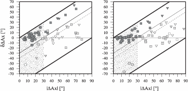
The mean difference |Ax| is zero for identical axes’ orientations. Interchanging two axes
(for example changing a normal to a thrust or a left lateral to a right lateral mechanism) results
in |Ax| = 60o. We thus require A quality solutions to have |Ax|< 30o; solutions with
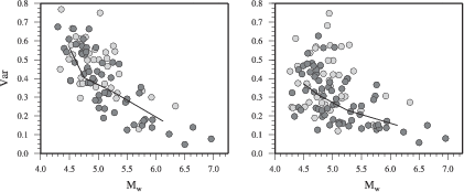
|Ax| > 30o are either B or C quality, depending on the magnitude difference (Figure 3.3).
Figure 3.4 (top) shows the distribution of |Ax|. For quality A solutions the mean
value of |Ax| is 18.8o ± 6.7o. Two solutions with |Ax|< 30o are not quality A,
because one violates the depth (quality B) and one the magnitude criterion (quality
C).
We also checked the focal parameter agreement between the SAMT and SRMT catalogs
using the radiation pattern coefficient  P (Kuge & Kawakatsu, 1993), a parameter describing
the radiation pattern similarity of two mechanisms. Our median P = 0.85 for A quality
solutions compares well with the median of P = 0.88 found by Helffrich (1997) who compared
ERI, Harvard and USGS catalogs for shallow earthquakes (most SAMTs are for shallow
earthquakes).
P (Kuge & Kawakatsu, 1993), a parameter describing
the radiation pattern similarity of two mechanisms. Our median P = 0.85 for A quality
solutions compares well with the median of P = 0.88 found by Helffrich (1997) who compared
ERI, Harvard and USGS catalogs for shallow earthquakes (most SAMTs are for shallow
earthquakes).
Because of the low-depth resolution and the discrete set of trial depths, we require that the
difference |z| between SAMT depth range (best-fit depth plus uncertainty) and SRMT depth
is < 10 km for an A quality solution. A similar scheme was proposed by Kubo et al. (2002)
when comparing the Japanese regional NIED catalog with the Harvard-CMT and the Japanese
Meteorological Agency (JMA) focal mechanism catalog. Differences |z| > 10 km result in
B or C solutions (Figure 3.3). Figure 3.4 (middle) shows |z| for the three quality
groups.
The difference between SAMT and SRMT Mw estimates must be < 0.2 units for an A or B
quality solution (Mw =  - 10.73 following Kanamori (1977)). A required difference
|Mw|< 0.2 is consistent with Pasyanos et al. (1996), who found that automatic and revised
regional MT solutions in northern California have Mw estimates that usually differ by less than
0.2 units even when the focal mechanism and depth estimates differ strongly. Mw depends
mainly on the signal amplitude and is therefore the parameter easiest to resolve. One goal for
our automatic procedure is to provide robust Mw values so that disaster relief agencies may
quickly estimate possible earthquake damages. Damages are governed by the rupture
process and local site effects; our Mw can only help to estimate whether no, local or
widespread damages are expected. Therefore we accept an Mw estimate as accurate
even when the focal mechanism and/or the depth exceed their A-quality threshold:
these are our quality B solutions. |Mw| > 0.2 are quality C, irrespective of focal
mechanism and depth (Figure 3.3). The distribution of |Mw| is shown in Figure 3.4
(bottom).
- 10.73 following Kanamori (1977)). A required difference
|Mw|< 0.2 is consistent with Pasyanos et al. (1996), who found that automatic and revised
regional MT solutions in northern California have Mw estimates that usually differ by less than
0.2 units even when the focal mechanism and depth estimates differ strongly. Mw depends
mainly on the signal amplitude and is therefore the parameter easiest to resolve. One goal for
our automatic procedure is to provide robust Mw values so that disaster relief agencies may
quickly estimate possible earthquake damages. Damages are governed by the rupture
process and local site effects; our Mw can only help to estimate whether no, local or
widespread damages are expected. Therefore we accept an Mw estimate as accurate
even when the focal mechanism and/or the depth exceed their A-quality threshold:
these are our quality B solutions. |Mw| > 0.2 are quality C, irrespective of focal
mechanism and depth (Figure 3.3). The distribution of |Mw| is shown in Figure 3.4
(bottom).
For our data we observe that SAMTs with |Ax|< 30o usually have |z|< 10 km and
|Mw|< 0.2. Based on our rules, the 87 automatic moment tensors are divided into 38 quality
A, 21 quality B and 28 quality C solutions.
3.4.2 Automatic assigned quality
The true quality can be verified only a posteriori. For automatic solution dissemination, we
derive empirical rules, matching the a posteriori true qualities that can be implemented into the
automatic procedure. The rules follow three principles: (1) applied to the whole data set, the
rules should closely follow the true quality; (2) the rules should not overestimate quality: true
quality B solutions should not be assigned Aa, and quality C should not be assigned
Aa or Ba (we use the superscript a to denote assigned quality). We want to have
high confidence that an automatic Aa solution is truly A; (3) the rules should be
simple.
A combination of number of stations and components used (i.e., with good signal-to-noise
ratio) provides a simple yet reasonably accurate measure to assess solution quality (Table 3.2).
The empirical rules were defined based on the April 2000 to April 2002 data set and may be
modified when, for example, station availability increases. Figure 3.5 shows that it is
generally sufficient to use 2 or more components for each station to obtain quality
A solutions even when only a few stations can be used. Using fewer stations and
components results in lower quality solutions. Many solutions of earthquakes located in the
larger Iran area result in quality B or C, because of the few stations available. For the
southern Aegean Sea (34o < Lat. < 38.5o; 20o < Long. < 30o) we observe an interesting
difference: we need more stations and components to obtain true quality A solutions
(Figure 3.5). This exception is possibly due to large event-station distances (Figure
3.2).
| Table 3.2: | Empirical rules applied to derive assigned quality. Number of stations (St) and
components (Co) used characterize solution quality (Figure 3.5). Rules for earthquakes
located in the southern Aegean Sea (34o < Lat < 38.5o; 20o < Long < 30o) are slightly
different (right): there, a larger number of stations is required to obtain assigned quality
A. |
|
|
| | Quality | Rules | Rules |
| | (Europe-Mediterranean) | (Southern Aegean Sea) |
|
|
| | A | St > 10 & Co/St > 1.5 | St > 16 & Co/St > 1.5 |
| | St > 5 & Co/St > 2 | |
| | St > 3 & Co/St = 3 | |
|
|
| | B | All other solutions | All other solutions |
|
|
| | C | Co < 7 | Co < 7 |
|
|
| | |
|
The empirical rules were designed to not overestimate true quality. Underestimating a few
events is implicitly allowed and results in fewer assigned quality Aa and Ba solutions
compared to true quality. Undesired upgrade happens only for 2 events from B to
Aa (6% of 34 assigned quality Aa solutions) and 3 events from C to Ba (14% of 22
assigned quality Ba solutions). No true C event is assigned to Aa. Such upgrades
are confined to smaller events (Mw < 5.3). The empirical rules actually reproduce
82% of the true quality data set; most differences (11 events) are caused by quality
downgrade. Based on these observations, we have high confidence that our automatically
disseminated solutions cause few (or no) false alerts for large, potentially damaging
earthquakes.
3.5 Discussion
3.5.1 Performance
In this section we focus on the geographical event distribution and factors that cause low true
quality solutions. We also compare our Mw, depths and focal mechanisms results with the
SRMT, the Harvard (CMT) and INGV (MEDNET) moment tensor results to illustrate their
high consistency.
The distribution of the analyzed events (circles, Figure 3.2) reflects long-term seismicity
(Jackson & McKenzie, 1988). The distribution of high quality solutions, however, is also
affected by the station distribution (black triangles, Figure 3.2). Generally, analysis is hampered
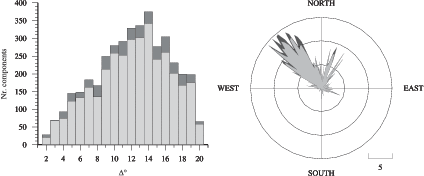
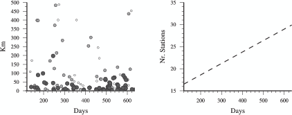
by long average event-station distances (Figure 3.6). Most data come from stations at distances
> 7o with a peak around = 14o - 15o caused by high seismicity in the Aegean Sea and
high station density in central Europe. Most high quality solutions are produced for
earthquakes in the central-eastern Mediterranean region, where data from stations
in central Europe, Israel, the Caucasus region and Russia provide good azimuthal
coverage. In the western Mediterranean region, seismicity is relatively low and the
inadequate station distribution resulted in a quality B solution for the one event
analyzed. Station coverage for events in the Caspian Sea and Zagros mountain regions
is also low and few of the frequent events have well-recovered source parameters.
In central and northern Europe we obtained few high quality automatic solutions.
Although a large number of stations is available, there, the lowpass filter at 50 s
precludes moment tensor retrieval for the typically smaller (Mw < 4.5) events of this
region.
Not all events triggered by our automatic procedure resulted in a moment tensor. Triggered
events result in no-solution when either (1) no data are available, (2) the automatic alert is a
false alarm, (3) the epicenter is strongly mislocated, (4) the true magnitude is far lower than the
alert magnitude or when any of these cases combine. Case (4) caused most no-solution events
due to the low trigger-threshold set for analysis (M > 4.7), that assures the processing of all
stronger events. We let the procedure decide whether a solution can be produced or not. For a
few smaller events, few traces containing only long-period noise were inverted, resulting in
quality C solutions.
Earthquake size is the most stable source parameter and a few, good signal-to-noise
seismograms generally constrain the seismic moment Mo. Figure 4.12 shows the high correlation
of the automatic Mw estimates relative to SRMT, CMT and MEDNET Mw’s. Mean differences
are very small,  < 0.02 relative to SRMT and CMT, and lower than 0.1 unit relative to
MEDNET, with standard deviations close to 0.1. The linear regressions (dashed lines in
Figures 4.12) have slopes close to 1 and small intercepts, roughly consistent with a
one-to-one relation between the magnitude estimates. We did not interpret small
apparent differences because the data set is too small. Mean differences and regressions
were determined for A and B quality solutions combined, because we did not see any
significant systematic difference in the A and B quality Mw estimates (Figure 3.4
bottom).
< 0.02 relative to SRMT and CMT, and lower than 0.1 unit relative to
MEDNET, with standard deviations close to 0.1. The linear regressions (dashed lines in
Figures 4.12) have slopes close to 1 and small intercepts, roughly consistent with a
one-to-one relation between the magnitude estimates. We did not interpret small
apparent differences because the data set is too small. Mean differences and regressions
were determined for A and B quality solutions combined, because we did not see any
significant systematic difference in the A and B quality Mw estimates (Figure 3.4
bottom).
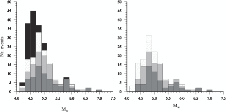
Quality A solutions were obtained for earthquakes from Mw = 4.5 to Mw = 7.0. In general
larger events (Mw > 5.5) result in quality A solutions (Figure 3.8), and earthquakes with
Mw < 5.5 result in quality A or B. We obtained 3 quality B solutions for earthquakes with
Mw > 5.5; in all cases the lower quality was caused by the inaccurate quick location used for
the inversion. We repeated the inversion with the PDE-location. In two cases we obtained A
quality solutions. One case stayed B quality, because of |Ax| = 31o, just outside the A quality
criterion (|Ax|< 30o); the depth and magnitude differences both satisfied the A quality
criteria. The number of MT solutions and the ratio of A/B solutions decrease for earthquakes
with Mw < 5.0 due to lower signal strength and the large event-station distances (Figure
3.6).
Figure 3.9 illustrates the limitations of long-period (T > 50 s) analysis with respect to
magnitude or signal strength. Variance increases with decreasing event size, effectively setting
the lower limit for retrieving MT solutions to Mw  4.5. At such long periods signal strength at
smaller magnitudes is just slightly above the noise level. We also observe that variance for
quality B is higher than it is for A solutions.
4.5. At such long periods signal strength at
smaller magnitudes is just slightly above the noise level. We also observe that variance for
quality B is higher than it is for A solutions.
Long period surface waves offer only limited depth resolution (Giardini, 1992). However,
depth of quality A solutions agree very well with those in SRMT, CMT and MEDNET (Figure
3.10). The mean difference is always < 4 km with a standard deviation  < 15 km. Our
SAMT catalog contains only 3 deep earthquakes with quality A and we observe no significantly
greater depth estimate differences for these events. Events with large depth difference
(|z|> 20) are different events in each panel, reflecting the depth differences in the catalogs
used for comparison. Note that quality A solutions for shallow and deep earthquakes are always
correctly distinguished.
< 15 km. Our
SAMT catalog contains only 3 deep earthquakes with quality A and we observe no significantly
greater depth estimate differences for these events. Events with large depth difference
(|z|> 20) are different events in each panel, reflecting the depth differences in the catalogs
used for comparison. Note that quality A solutions for shallow and deep earthquakes are always
correctly distinguished.
Figure 3.11 shows the focal mechanisms of the true quality A solutions together with the
available SRMT, CMT and MEDNET solutions. Focal mechanisms show excellent agreement
for all earthquakes: shallow, deep, weak and strong. Larger differences exist for only 3 CMT
solutions (Nr. 20, 33, 36). These earthquakes are small (Mw = 5.0 - 5.1) for CMT analysis.
Their CMTs have large non-double couple parts (0.316 < < 0.342) and large relative
moment tensor uncertainties E (0.261 < E < 0.673) compared to the average values = 0.124
and E = 0.165 of all 19589 CMT solutions (1976 until November 2002). E is defined in Davis &
Fröhlich (1995). Moment tensors with high and E have poorly constrained focal parameters
(Fröhlich et al., 1997).
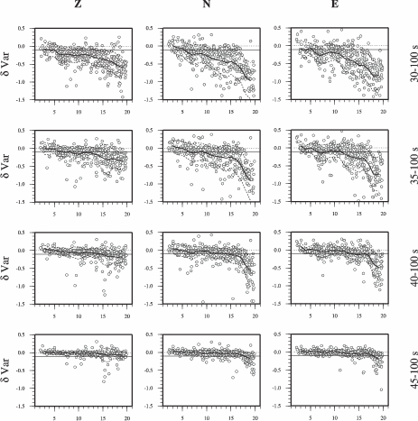
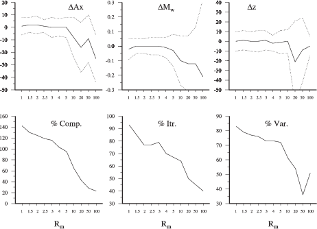
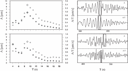
3.5.2 Frequency band and location
Our goal is to retrieve as many quality A solutions as possible, even for smaller earthquakes
(4.5 < Mw < 5.0), while minimizing the number of quality C solutions. Solution quality
depends on station distribution, location accuracy and the ability to correctly match phases in
the seismograms. For the given station distribution (Figure 3.2), we performed two tests. First,
we tried to find the optimum frequency band for analysis with the quickly available locations
and data set used for near real-time processing. The frequency band needs to match phases -
easy at longer periods - and contain good signal-to-noise seismograms - higher at shorter
periods. We thus performed inversions for 5 selected period ranges (40 - 60, 45 - 80, 50 - 100,
60 - 125, and 70 - 140 s). In a second step, we repeated the same analysis with the more
accurate PDE-locations to see whether location accuracy affects the choice of frequency
band.
The number of quality A, B and C solutions changes strongly with different frequency bands
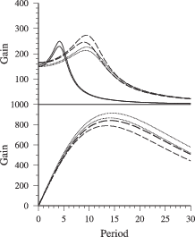
(Figure 3.12, top left). The largest number of quality A solutions (and highest ratio of A/C
solutions) is obtained with the 50 - 100 s band for the quickly available locations. Using the
more accurate PDE-locations, the optimal period range shifts to lower periods of 45 - 80 s
(Figure 3.12, bottom left). The reason for this shift is that mislocation introduces errors in the
initial phase that are then mapped onto the moment tensor. The effect is smaller at longer
periods (Patton & Aki, 1979) and the accuracy of the quick locations sets the optimum period
range to 50 - 100 s. At longer periods (60 - 125, 70 - 140 s) the number of quality
A and B solutions decreases for the quick and the PDE-locations because of weak
signals for the smaller events. At these period ranges, only stronger earthquakes can be
analyzed.
For shorter periods (40 - 60 s), the number of quality A solutions decreases strongly even for
the PDE-locations. In most cases, quality A solutions at 45 - 80 s (or 50 - 100 s) become B at
40 - 60 s (Figure 3.12, bottom left). At periods below 50 s, surface waves become more sensitive
to crustal thickness and average crustal velocity variations so that significant travel-time
differences relative to PREM result (Larson & Ekström, 2001; Pasyanos et al., 2001).
Unresolved near-source earth structure may also cause surface wave amplitude anomalies
(van der Lee, 1998). Both phase and amplitude differences limit reliable moment tensor
retrieval below 50 s period for our uneven station distribution and our average event-station
distances of about 1500 km.
The frequency band chosen has little effect on the overall quality of the focal mechanism and
depth estimates for quality A solutions. This also holds for the Mw estimates for A and B
solutions measured relative to SRMT (Figure 3.12). The median values of the radiation pattern
coefficient P are generally high, close to the value found by Helffrich (1997), and decrease
only slightly for shorter periods. There is no significant change for the mean depth
difference; all means are < 3 km with standard deviations < 15 km. Magnitude Mw
differences for quality A and B solutions are close to 0.0 unit with standard deviation
< 0.1.
From our tests, we deduce that the 50 - 100 s period range is the best average range with
the quickly available locations for the entire European-Mediterranean region. It allows routine
MT analysis for earthquakes down to Mw 4.5.
3.5.3 Current improvements
Two factors limit automatic retrieval of well-resolved MT for Mw > 4.5 earthquakes:
location accuracy (Figure 3.12), usually lower for smaller events (Mw < 5.0) and
the limited, inhomogeneous distribution of near real-time accessible stations (Figure
3.2).
Location accuracy is more important for shorter period analysis. Accurate quick locations
are starting to become routinely available from the European-Mediterranean Seismological
Center (EMSC). The EMSC merges automatic arrival-time picks from several European
institutions, and the virtual network’s improved station coverage and aperture is capable of
accurate automatic locations (Bossu et al., 2002). The locations we have received since June
2002 are of good quality.
The geographical distribution of near real-time accessible broadband stations is limited and
inhomogeneous (Figure 3.2). In the context of the European MEREDIAN project (van
Eck et al., 2001), the ORFEUS data center now has near real-time access to an
increased (and still growing) number of broadband stations. Their distribution (white
triangles, Figure 3.2) partially fills gaps like the western and central Mediterranean Sea,
Turkey and eastern Europe. Northern Africa, however, lacks sufficient broadband
instruments. For events since mid-2002, these data are available to us. Preliminary
scanning of the results shows that the smaller epicentral distances overall and improved
azimuthal coverage already increased the number of quality A relative to quality B and C
solutions.
Better quick locations and a denser network (and the resulting reduced epicentral
distances) also may speed up analysis and lower magnitude thresholds in the future. For
closer epicentral distances, 15-minute seismograms contain the entire surface wave
train. Reducing the seismogram length by 50% and assuming faster data accessibility,
automatic solutions could then be obtained within 45 - 60 min after an event. At closer
epicentral distances, signal strength is larger and relatively less perturbed by crustal and
upper mantle heterogeneities. Combined with analysis at shorter periods, we would
expect more reliable source parameter estimates for smaller events than possible
now.
Although improved EMSC locations and additional data from ORFEUS started becoming
available in mid-2002, we did not include these more recent events here. We wanted to have
constant conditions - location and data access - for the entire period covered in this paper and
therefore did not mix the two intervals.
3.6 Conclusions and outlook
We presented a fast and fully automatic procedure for moment tensor retrieval of moderate to
strong (Mw > 4.5) earthquakes in the European-Mediterranean region using long-period
(50 - 100 s) regional ( < 20o) seismograms. Automatic solutions are currently available within
90 minutes after an event. From April 2000 to April 2002, we obtained 87 moment tensor
solutions that we grouped into three qualities based on main stress axes’ orientation, depth and
Mw similarity with an independent, high quality moment tensor catalog. For 38 quality A
solutions, magnitude, depth and focal mechanisms are well-resolved; 21 B solutions have
well-resolved magnitude; 28 C solutions are not reliable. We derived simple empirical rules
based on the number of stations and components used to predict the quality of a solution
without a seismologist’s interference. Automatic quality Aa MTs are disseminated to EMSC
(http://emsc-csem.org), quality Aa and Ba solutions are displayed on our web page
(http://www.seismo.ethz.ch/mt), Aa and Ba solutions can be obtained via e-mail (contact first
author for details).
In the near future, we foresee largely improved near real-time automatic waveform analysis
capabilities and successful routine MT applications to smaller earthquakes (Mw 4.0) for most
of the European-Mediterranean region. Many national networks are transitioning to BB stations
with near real-time data transmission. Connecting these national data centers via internet will
create a dense European-wide virtual network that could be used, for near real-time event
detection, size determination and MT inversion in the European-Mediterranean region. We can
realize this scenario by increasing both the number of BB stations, particularly where no or few
stations currently exist, and near real-time open access to these data for the scientific
community.
Acknowledgments
We thank Daniel Stich and an anonymous reviewer for their constructive comments. We thank
Suzan van der Lee and Yuan Gao for providing modified moment tensor analysis codes. We
appreciate discussions with Günter Bock about the topic, we will miss him. We thank Kathleen
J. Jackson for enhancing the manuscript by correcting our grammar. Most figures were
produced with GMT (Wessel & Smith, 1995). High quality near real-time broadband data
were obtained from the following institutions and networks: GEOFON, Potsdam
(Germany); Gräfenberg Seismological Observatory, Erlangen (Germany); Institute of
Physics of the Earth, Masaryk University, Brno (Czech Republic); MEDNET, Istituto
Nazionale di Geofisica e Vulcanologia, Roma (Italy); National Data Center, Soreq (Israel);
Zentralanstalt für Meteorologie und Geodynamik, Wien (Austria); and the additional
members of the MEREDIAN consortium and its lead agency ORFEUS, De Bilt (The
Netherlands). Quick earthquake locations are send to us by EMSC (France); Geol.
Survey B-W, Freiburg (Germany); GERESS array (Germany); GSR, Obninsk (Russia);
IGN, Madrid (Spain); INGV, Rome (Italy); IPRG, Tel Aviv (Israel); LDG, Paris
(France); NEIC (USGS); NIEP, Bucharest (Romania); SDAC, Hannover (Germany); (see
http://www.seismo.ethz.ch/redpuma).
Chapter 4
Automatic moment tensor analysis of moderate earthquakes
4.1 Summary
I present an improved automatic Frequency Adaptive Regional Moment Tensor (FARMT)
routine. FARMT computes moment tensors (MT) of events with magnitude down to Mw 4.3
in the European - Mediterranean area using complete surface wave seismograms recorded at
regional distances ( < 20o). Two features lead to significant improvements of FARMT
compared to the original standard routine (SR) for 4.3 < Mw < 4.7 events. First, the
short-period cut-off at each station depends on station-event distance. Second, FARMT
performs a signal-to-noise analysis to remove noisy traces and period-bands that do
not exceed a minimum signal-to-noise ratio Rm. Tests performed to asses the short
period cut-off and Rm for automatic FARMT indicate that the short period cut-off for
events in the eastern Mediterranean Sea and the near East is 50 s. Events in Europe
can be analyzed with a distance-variable short period cut-off ranging from 35 s for
the closest to 50 s for distant stations. Values of Rm = 1 - 5 lead to well resolved
mechanisms and use more seismograms for inversion than the standard method. The
automatic FARMT uses Rm = 2, since it assures usage of seismograms with weak,
often nodal signal, and reduces the number of iterations by about 20% to reach the
final MT. For the May 2002 to September 2003 data-set, the automatic FARMT
resulted in 66 solutions with well determined MT, which is a 20% increase relative to
SR.
4.2 Introduction
Since April 2000, the Swiss Seismological Service (SED) computes real-time and fully automatic
moment tensor (MT) solutions for Mw > 4.5 earthquakes in the European-Mediterranean area
(Bernardi et al., 2004). Moment tensors are computed using 50 - 100 s period surface waves
recorded at regional distances ( < 20o). For stronger events (M
w > 5.5) the complete moment
tensor (seismic moment Mo, depth and focal mechanism) is generally well resolved. For
4.5 < Mw < 5.5 events, Mo is generally well resolved while depth and focal mechanism
resolution decreases with decreasing event size. Goal of this work is to improve the
results for 4.5 < Mw < 5.5 events and to extend automatic analysis to even smaller
events.
Fast and reliable MT analysis for moderate events in densely populated areas like central
Europe is becoming a necessity for the seismological community to provide rapid information to
the public. An example is the recent Mw = 4.5 February 23, 2004 Rigney, eastern
France, event, that was felt over the entire western part of Switzerland. Within minutes
the press and a large number of concerned people called the SED or connected to
the SED’s web-page looking for information about the event. In addition to rapid
information, efficient automatic MT analysis for Mw >~126' 4.5 events will relatively quickly
lead to a MT catalog, even in areas with low seismicity, like most of the European -
Mediterranean region that is indispensable for seismic hazard and seismotectonic
studies.
The current routine - called standard routine (SR) here - satisfactorily analyzes only few
events with Mw  4.8, because analysis is performed at a fixed period band of 50 - 100 s. The
50 - 100 s interval is the best single period interval for automatic MT computation in European
and Mediterranean region (Bernardi et al., 2004), considering the sparse set of near-real time
accessible stations, the limited accuracy of quick locations, and the complicated tectonic
setting.
4.8, because analysis is performed at a fixed period band of 50 - 100 s. The
50 - 100 s interval is the best single period interval for automatic MT computation in European
and Mediterranean region (Bernardi et al., 2004), considering the sparse set of near-real time
accessible stations, the limited accuracy of quick locations, and the complicated tectonic
setting.
However, since 2002 the number of near-real time data has significantly increased in the
European - Mediterranean region. Many of these stations are part of the Virtual European
Broadband Seismograph Network (van Eck et al., 2004) and data can be collected in near-real
time from the ORFEUS data-center. Accuracy of quick automatic locations for M > 4.5 events
has significantly increased in the European - Mediterranean region because more stations
contribute data resulting in a relatively dense, large aperture European network. The quick,
more accurate locations, provided by EMSC (Maset-Roux & Bossu, 2004) and by ORFEUS
(van Eck et al., 2004), together with the VEBSN data are key factors for automatic MT
analysis of moderate events.
In this chapter, I present a modified procedure, which significantly lowers the magnitude
threshold for automatic MT analysis toward Mw 4.3. For such small events, signal energy
above 50 s is generally weak and MT analysis requires inclusion of shorter periods. Although
more near-real time broad-band stations exist, improving azimuthal coverage and lowering
event-station distances, the distribution is still not homogeneous resulting in event
data-sets that include near and far stations. Thus, I derived a distance dependent short
period cut-off, which allows an optimal period band setting for MT inversion using
near and far stations simultaneously (Section 4.3). An additional short and/or long
period cut-off depending on the signal-to-noise ratio is applied to remove those periods
without sufficient signal (Section 4.4). The notation from chapter 3 is kept, quality A
solutions have well resolved Mo, depth and focal mechanism, quality B only well resolved
Mo, and quality C is not reliable. Quality is assessed relative to SRMT (Braunmiller
et al., 2002).
4.3 Distance dependent short period cut-off
The standard routine SR uses a short period cut-off at 50 s for all event-station distances,
ensuring synthetics and observed seismograms are in phase even for large distances ( 20o).
At shorter distances, PREM synthetics can probably be used at shorter periods (Braunmiller
et al., 2002). The test data-set consists of 20 events covering the entire European -
Mediterranean region . The data-set includes crustal and intermediate deep events and covers
the magnitude range 4.5 < Mw < 6.7. The automatic SR resulted in quality A solutions for
each event, implying that a sufficient number of seismograms (from 39 to 115) could be
used for inversion in the 50 - 100 s pass band. The automatic moment tensors were
then revised using the PDE-location, to exclude low quality waveform fit because of
inaccurate locations. These solutions are used as reference (Table 4.1 and Figure
4.1).
| Table 4.1: | Reference events used to calibrate the distance dependent short period cut-off.
For each earthquake the event origin time and coordinates from PDE, and depth in [km],
Mw, and MT derived fault plane orientations are listed . |
|
|
|
|
|
|
|
|
|
|
|
|
|
| | Event Lat. | Long. | z | Mw | Plane 1 | Plane 1
|
|
|
|
|
|
|
|
|
|
|
|
|
|
| | | | | | | | | | | | | | | |
|
|
|
|
|
|
|
|
|
|
|
|
|
| | 2000 | 04 | 06 | 00:05 | 45.72 | 26.58 | 125 | 5.05 | 343 | 31 | 29 | 227 | 75 | 117 |
| 2000 | 06 | 06 | 02:39 | 40.69 | 32.99 | 18 | 6.06 | 356 | 50 | -49 | 122 | 54 | -128 |
| 2000 | 06 | 13 | 01:41 | 35.15 | 27.13 | 25 | 5.36 | 228 | 75 | 4 | 137 | 85 | 165 |
| 2001 | 05 | 24 | 17:31 | 45.75 | 26.46 | 150 | 5.20 | 355 | 38 | 48 | 224 | 62 | 118 |
| 2002 | 02 | 03 | 07:08 | 38.49 | 31.31 | 18 | 6.60 | 243 | 26 | -114 | 90 | 66 | -78 |
| 2002 | 09 | 06 | 01:18 | 38.39 | 13.71 | 14 | 5.94 | 35 | 46 | 61 | 253 | 50 | 116 |
| 2002 | 10 | 31 | 10:30 | 41.78 | 15.01 | 18 | 5.79 | 265 | 64 | -177 | 174 | 87 | -25 |
| 2002 | 11 | 01 | 15:06 | 41.76 | 14.85 | 18 | 5.76 | 261 | 58 | -175 | 169 | 86 | -31 |
| 2003 | 02 | 22 | 20:38 | 48.35 | 6.80 | 18 | 4.78 | 162 | 40 | -67 | 314 | 52 | -107 |
| 2003 | 03 | 29 | 17:39 | 43.15 | 15.51 | 10 | 5.52 | 307 | 34 | 124 | 88 | 62 | 69 |
| 2003 | 04 | 10 | 00:37 | 38.22 | 26.94 | 14 | 5.75 | 243 | 67 | 177 | 333 | 87 | 23 |
| 2003 | 04 | 11 | 09:24 | 44.82 | 9.09 | 18 | 4.87 | 296 | 72 | -167 | 203 | 78 | -17 |
| 2003 | 05 | 21 | 18:40 | 37.04 | 3.74 | 10 | 6.74 | 63 | 35 | 48 | 290 | 63 | 115 |
| 2003 | 05 | 29 | 02:12 | 36.82 | 3.36 | 14 | 4.98 | 188 | 80 | 5 | 97 | 84 | 170 |
| 2003 | 06 | 01 | 15:42 | 41.66 | 14.83 | 25 | 4.54 | 250 | 83 | -178 | 160 | 88 | -6 |
| 2003 | 07 | 06 | 19:07 | 40.45 | 26.07 | 18 | 5.81 | 350 | 57 | 7 | 256 | 83 | 147 |
| 2003 | 07 | 13 | 01:45 | 38.27 | 39.03 | 25 | 5.66 | 343 | 71 | -171 | 250 | 81 | -19 |
| 2003 | 07 | 26 | 08:33 | 38.03 | 29.05 | 18 | 5.48 | 319 | 54 | -14 | 58 | 78 | -143 |
| 2003 | 08 | 14 | 05:11 | 38.70 | 20.67 | 25 | 6.24 | 194 | 72 | -177 | 104 | 88 | -17 |
| 2003 | 08 | 14 | 16:14 | 38.86 | 20.44 | 18 | 5.47 | 0 | 31 | 102 | 175 | 59 | 82 |
| 2003 | 09 | 14 | 21:39 | 44.39 | 11.51 | 25 | 5.29 | 247 | 33 | 77 | 82 | 57 | 98 |
|
|
|
|
|
|
|
|
|
|
|
|
|
| | |
|
The test consists of observing the variance increase of each seismogram component relative
to its standard solution variance for different short-period cut-offs. In practice, I recomputed the
MT for each reference event changing the short-period cut-off only for one station per inversion
run while keeping the 50 - 100 s band for all other stations. Re-computation was used to check
whether shorter period synthetics are correctly realigned. With this approach, the MT solution
remains effectively unchanged, because one station does not influence the results based on a
large data-set. I tested short-period cut-offs of 30, 35, 40 and 45 seconds. The long period
cut-off was kept at 100 s. I did not test shorter periods, used often for manual regional MT
inversion (Braunmiller et al., 2002; Stich et al., 2003), because of the sparsity of close-by
stations and the requirements of the procedure to produce stable results in a fully automatic
fashion.
A waveform fit example is shown in Figure 4.2. The waveforms are the vertical components
of stations ISP ( = 2.80) and DIX ( = 16.40) for the M
w = 5.8 April 10, 2003 Turkey event.
For station ISP, the waveform fit remains good even for short period cut-offs of T = 30 - 35 s.
For DIX, the fit decreases significantly for periods T < 40 s. The waveform fit at a given short
period cut-off depends on epicentral distance. This general behavior is caused by limitations
imposed by the PREM model which is used throughout the study area for synthetic seismogram
calculation.
Figure 4.3 shows the normalized variance difference for each short period cut-off as
a function of epicentral distance for all components (at least 441 observations per
component) relative to the 50-100 fit. The mean (solid line) and standard deviation
(dashed lines) are moving window values with 1o steps using all data-points in the
surrounding ±1o distance. Figure 4.3 shows that the variance difference increases for longer
epicentral distances (from left to right in each panel) and for shorter period cut-offs
(from bottom to top in each column). This effect is slightly stronger for horizontal
components, probably because of the higher noise levels and possibly anisotropy.
The components are not rotated to transversal/radial and polarization anisotropy
observed in the Mediterranean region (Marone et al., 2004) affects both horizontal
components.
The variance difference increases smoothly over the = 20 - 200 distance interval. I
arbitrarily fixed the distance interval where the mean normalized variance difference does not
decrease more than -0.1 units for one of the three components. Based on Figure 4.2, even larger
variance increases appear to provide adequate fits (and thus MT solutions), however, the small
0.1 value ensures stable automatic results. All components have the same distance range for the
sake of simplicity. Based on this definition, the 30 s short period cut-off could be applied only
for distances < 30, were only few data are available. I thus selected 35 seconds as the shortest
cut-off period. Table 4.2 lists the resulting distance - short period cut-off setting
(T2). Table 4.2 also shows the standard 50 - 100 s pass-band for all distances (T0),
and two additional settings, which deviate slightly from T2: T1 is a more and T3 is
a less conservative setting. For full evaluation of the Ti cut-offs, I applied all four
settings to a 17 month data-set in the European - Mediterranean area (section 4.5)
combined with the signal-to-noise ratio dependent period band cut-off derived in the next
section.
| Table 4.2: | Summary of the period band - distance sets. T0 refers to the standard routine
that uses a 50 s short period cut-off for all distances. T2 is derived from Figure 4.3, while
T1 and T3 are derived from T2. |
|
4.4 Signal-to-noise ratio cut-off
The standard procedure uses a 100 s long period cut-off to compute the MT. When the
seismogram contains only noise or when the signal is above the noise only for periods shorter
than 100 seconds, the normalized variance of the station component is high. In the SR such
traces are removed iteratively (Bernardi et al., 2004).
Goal of this section is to implement a more straightforward approach to remove noisy traces.
With the following signal-to-noise ratio analysis the period band where the ratio exceeds a value
Rm are identified and selected for MT inversion.
This approach has two main consequences. First, when the epicentral distance criteria, for
example, indicates that the 50 - 100 s period range should be used for MT inversion and if the
signal-to-noise ratio of that trace does not exceed Rm for the entire range, the seismogram will
be removed from the data-set. This reduces the number of iterations and shortens the
computing time. Second, using only the period range where the data exceed Rm, for instance
from 50 s to 70 s, lowers the variance and the seismogram is used for inversion. The resulting
data-set for automatic MT inversion contains more traces than the SR, which is important for
moderate events analysis, where generally only few traces with good signal-to-noise ratio
exist.
The signal-to-noise ratio is determined by simple division of signal and noise power spectral
density for each sampled frequency. All seismograms have 1 second sampling interval and are
zero-padded to 2048 points. A 9-point smoothing is applied to the resulting power spectral
density curve.
The noise is characterized by non-stationary behavior with large variations between the low
and high noise levels for 10 - 100 s period waves (Peterson, 1993). Examples of noise variations
are shown in Figure 4.4, using a typical long period high noise (station MMLI, NS-component)
and low noise seismogram (station MOA, Z-component). The seismograms are divided into
fourteen 200 second long sub-windows, and for each window the power spectral density (dotted
lines on the right side, Figure 4.4) is computed. In both cases, the power spectral density varies
by about one order of size over the entire 10 - 100 s band within the short 1500 s noise
window.
The noise power spectral density PN is computed from the 200 s window before the P-wave
arrival to have a representative pre-signal noise estimate. A 200 s window, of course, does not
allow to solve single frequency features between 0.01 and 0.03 Hz. The goal of this analysis is
not to obtain a high single frequency resolution of the noise, where a very long time series
is needed, but to obtain an overall estimate of the noise level over a finite period
band. A short 6 point hanning taper is applied to each seismogram to remove edge
effects.
The signal power spectral density PS is computed from a window starting at the P-wave
arrival and ending with the 30 second group velocity surface waves. Since the earthquake alerts
that trigger the automatic procedure may not be correctly located (Bernardi et al., 2004), PS
analysis requires windows wide enough to contain the signal even when severe mislocation
occurred. The alert that triggers the procedure is not necessarily the location used for later
inversion, but for rapid data preparation I use the initial location for signal-to-noise-analysis.
Thus, I assume a maximum uncertainty of 200 km. P-wave (Kennett & Engdahl, 1991) and
surface wave group velocities (Larson & Ekström, 2001; Pasyanos et al., 2001; Cotte &
Laske, 2002) may also vary significantly within the European-Mediterranean area. I used
conservative fast V p = 8.5 km/s and slow 30 s group velocity V 30 = 2.5 km/s, to avoid
truncation of the signal. At each end of the signal window, I add 5% to apply a 5%
hanning taper to the seismogram without cutting into the data. The window length for
PS is long for far stations because of uncertainties. The signal length, that actually
contributes mostly to the power spectral value is shorter. I thus normalize PS for a 200 s
window.
To find the minimum signal-to-noise ratio required, I recomputed the MT of 14
4.4 < Mw < 5.0 events (Table 4.4). I also re-analyzed the Mw = 7.0 May, 2003 northern Algeria
event to verify that the signal-to-noise ratio analysis does not affect well resolved MTs of large
events. All 15 test events have accurate automatic location compared to their PDE-location; 12
are A-quality and 3 are B-quality solutions, using the SR. The actual period band used for
inversion is defined by the minimum signal-to-noise ratio Rm(f) = PS/PN. Only
seismograms that exceed Rm for a period band at least 15 s between 50 - 100 s are
selected.
Tested values of Rm are 1, 1.5, 2, 2.5, 3, 4, 5, 10, 20, 50 and 100. Figure 4.5, as an example,
shows the NS-component of station OBKA ( = 3.4o) for the May 10, 2003 Northwestern
Balkan Mw = 4.4 event. PS (thick black line), PN (thin black line) and the resulting
signal-to-noise ratio R (dotted line) are plotted. In the time domain, the signal is visible in the
35 - 60 filtered seismogram (right side, middle), while at longer periods (right side,
bottom), only noise is visible. The period-band for MT inversion for this component is
50 - 80 seconds when Rm = 1 or 50 - 57 seconds when Rm = 2. In the second case the
component is not used because the window width of usable signal length is less then 15 s
wide.
To select the ”best” value of Rm, I analyzed the solution stability, the number of
seismograms used, the solution fit and the reduction of iterations as a function of Rm relative
to the standard solution. Figure 4.6 summarize the average performance for the 15
events. Stability of the solution is manifested by small changes in the principal axes
orientation Ax (Bernardi et al., 2004), moment magnitude Mw and depth z. For
Rm < 5, Ax and Mw are small indicating stable solutions. Depth resolution does
not seem to depend strongly on Rm. For Rm > 5 the number of components used
(bottom, left) is less than for the standard solution; one goal of the signal-to-noise
analysis is to use more data to be able to analyze smaller event, so Rm > 5 is not
acceptable. Using fewer data may explain the increase of Ax and Mw for Rm > 5. The
number of iterations and the normalized variance decrease steadily. Because of the
fewer components used, the resulting solutions are actually less well resolved. Using
large Rm values (Rm = 20 - 100), reduces the amount of data used significantly. For
Rm = 100 only 12 of 15 events still have any traces (i.e. for 3 events no traces are left for
inversion).
Based on Figure 4.6, the minimum signal-to-noise ratio can be set to values of 1 < Rm < 5. I
selected Rm = 2 for further analysis. With Rm = 2, the solutions are stable, more data ( 20%)
are used relative to the standard solution, fewer iterations ( 20%) are required and the
variance is significantly reduced ( 20%). The relatively small value of Rm = 2 ensures to use
small signals from nodal, far and relatively small events. Data that are still noisy and cannot be
fit are automatically removed by the variance criteria during the inversion (chapter
3).
4.5 Application to MT data-set
Between May 2002 and September 2003, the SR was triggered 246 times, 55 resulted in quality
A, 44 in quality B and 34 in quality C solutions (Table 4.4). 113 alerts did not result in a MT
because the earthquake was too weak, or the earthquake occurred outside our area of interest
or no data were available. For the same data-set, the MTs are recomputed using
the distance dependent short period cut-offs Ti (section 4.3, Ti = T0 - T3) and
signal-to-noise ratio Rm = 2 (section 4.4). Results are listed in Table 4.4. No event with
Mw < 4.2 resulted in an A or B quality solution, which is to be expected from the period
bands Ti considered. After removing these triggers our data-set consists of 169 events.
As for SR, not all events resulted in MT solution (maximum number is 139, Table
4.3).
| Table 4.3: | Table of the 139 automatic moment tensor solutions. From left to right: Event number, PDE-location, true and
assigned quality, seismic moment Mo in Nm, Mw, depth in km, orientation of the two fault planes in degree, number of
stations, components and quickly available location used for inversion. For completeness, we include all source parameters
even for true quality B and C solutions. For B, only size is well resolved and for C, none of the parameters is reliably resolved.
For further studies, use Mw, depth and focal mechanism from A and only Mw from B solutions. Events located in eastern
Mediterranean Sea and near East are computed using the T0-setting, all others using the T1-setting. Events marked with *
are used to set Rm (Section 4.4). |
|
|
|
|
|
|
|
|
|
|
|
|
|
|
|
|
|
|
|
|
|
|
|
| | Nr. | | Location (PDE) Quality | Mo | Mw | Depth | Plane 1 | Plane 2 | St. | Co. | Location used for inversion
|
|
|
|
|
|
|
|
|
|
|
|
|
|
|
|
|
|
|
|
|
|
|
|
| | | Date | Time | Lat | Long | True | Assigned | | | | Strike | Dip | Rake | Strike | Dip | Rake | | | Time | Lat | Long |
|
|
|
|
|
|
|
|
|
|
|
|
|
|
|
|
|
|
|
|
|
|
|
| | 1 | 02-05-03 | 08:13:10.3 | 85.972 | 31.14 | C | c | 5.23e+16 | 5.08 | 125 | 135 | 28 | 151 | 250 | 76 | 64 | 2 | 2 | 54.00 | 24.90 | 15:38:27.1 |
| 2 | 02-05-16 | 11:00:12.0 | 29.672 | 51.70 | C | c | 1e+16 | 4.60 | 200 | 331 | 78 | -168 | 238 | 78 | -11 | 2 | 2 | 28.80 | 51.20 | 11:01:01 |
| 3 | 02-05-17 | 15:52:20.9 | 29.589 | 51.96 | C | c | 1.15e+17 | 5.31 | 75 | 196 | 62 | 177 | 288 | 88 | 27 | 2 | 3 | 28.20 | 58.50 | 15:51:22.1 |
| 4 | 02-05-21 | 20:53:29.7 | 36.627 | 24.27 | A | a | 8.02e+17 | 5.87 | 75 | 351 | 79 | 8 | 259 | 81 | 168 | 11 | 30 | 36.70 | 24.50 | 20:53:29.0 |
| 5 | 02-05-24 | 20:42:26.8 | 44.761 | 21.61 | C | a | 2.1e+16 | 4.82 | 10 | 76 | 23 | -132 | 301 | 72 | -73 | 12 | 25 | 46.20 | 22.40 | 20:42:46.9 |
| 6 | 02-06-01 | 16:12:36.9 | 29.568 | 51.22 | C | c | 1.54e+17 | 5.39 | 75 | 181 | 38 | -165 | 80 | 81 | -52 | 1 | 1 | 26.60 | 58.20 | 16:11:19.8 |
| 7 | 02-06-06 | 22:35:41.0 | 35.648 | 26.18 | B | a | 6.38e+16 | 5.14 | 31 | 127 | 28 | -18 | 234 | 81 | 116 | 24 | 57 | 35.70 | 26.50 | 22:35:36.6 |
| 8 | 02-06-08 | 20:13:06.8 | 44.360 | 10.69 | A | a | 2.63e+15 | 4.22 | 31 | 282 | 33 | 80 | 113 | 57 | 96 | 10 | 18 | 44.50 | 10.80 | 20:13:00 |
| 9 | 02-06-18 | 03:19:24.3 | 33.326 | 45.91 | B | c | 1.9e+16 | 4.79 | 75 | 9 | 59 | -31 | 116 | 63 | 145 | 3 | 4 | 36.00 | 43.00 | 03:20:03 |
| 10 | 02-06-18 | 22:23:37.7 | 44.438 | 10.81 | A | c | 3.56e+15 | 4.30 | 31 | 109 | 44 | 81 | 301 | 45 | 98 | 2 | 3 | 44.60 | 10.80 | 22:23:43.0 |
| 11 | 02-06-22 | 02:58:21.3 | 35.626 | 49.04 | A | b | 7.78e+18 | 6.53 | 10 | 262 | 48 | 48 | 135 | 55 | 126 | 4 | 12 | 36.30 | 48.50 | 02:58:30.1 |
| 12 | 02-06-22 | 06:45:34.6 | 35.666 | 48.92 | B | c | 7.25e+16 | 5.18 | 42 | 237 | 34 | 58 | 94 | 60 | 110 | 3 | 4 | 32.30 | 50.40 | 06:45:06 |
| 13 | 02-06-22 | 14:27:16.0 | 35.497 | 48.97 | B | c | 9.04e+15 | 4.57 | 42 | 276 | 65 | -176 | 184 | 86 | -24 | 2 | 2 | 35.50 | 49.10 | 14:27:16.0 |
| 14 | 02-06-24 | 01:20:36.7 | 35.850 | 9.88 | A | a | 5.9e+16 | 5.12 | 10 | 352 | 39 | 73 | 193 | 52 | 103 | 16 | 34 | 35.80 | 9.90 | 01:20:35.0 |
| 15 | 02-07-16 | 06:56:25.5 | 33.883 | 24.15 | A | b | 1.87e+16 | 4.79 | 31 | 150 | 41 | 50 | 18 | 59 | 119 | 7 | 15 | 33.00 | 24.00 | 06:56:26.0 |
| 16 | 02-07-22 | 05:45:05.4 | 50.875 | 6.22 | A | a | 1.11e+16 | 4.63 | 25 | 287 | 43 | -106 | 128 | 48 | -75 | 7 | 16 | 51.20 | 5.80 | 05:44:59.2 |
| 17 | 02-07-28 | 17:16:31.1 | 37.932 | 20.69 | B | a | 5.55e+16 | 5.10 | 18 | 214 | 68 | 179 | 304 | 89 | 21 | 31 | 72 | 38.00 | 20.62 | 17:16:30.3 |
| 18* | 02-07-30 | 12:20:23.6 | 37.698 | 29.18 | A | a | 2.22e+16 | 4.83 | 31 | 126 | 27 | -75 | 289 | 63 | -97 | 14 | 17 | 38.00 | 28.90 | 12:20:28.0 |
| 19 | 02-08-06 | 06:16:18.9 | 37.980 | -1.89 | B | a | 5.93e+16 | 5.12 | 10 | 183 | 24 | -25 | 296 | 79 | 112 | 11 | 27 | 38.00 | 358.10 | 06:16:21.3 |
| 20 | 02-08-18 | 11:52:28.8 | 40.808 | 42.57 | B | b | 1.52e+16 | 4.72 | 18 | 77 | 48 | 122 | 213 | 50 | 58 | 9 | 10 | 41.10 | 40.60 | 11:52:42.4 |
| 21 | 02-09-02 | 01:00:03.3 | 35.701 | 48.83 | A | b | 8.8e+16 | 5.23 | 14 | 267 | 47 | 45 | 143 | 58 | 127 | 5 | 9 | 36.80 | 47.10 | 01:01:20.1 |
| 22* | 02-09-02 | 09:23:45.2 | 35.081 | 26.52 | A | b | 1.23e+16 | 4.66 | 31 | 22 | 29 | 51 | 244 | 67 | 109 | 8 | 10 | 35.02 | 26.04 | 09:23:49.1 |
| 23 | 02-09-05 | 22:19:51.5 | 38.720 | 24.53 | A | a | 3.47e+16 | 4.96 | 25 | 252 | 51 | -178 | 161 | 89 | -38 | 38 | 89 | 38.80 | 24.50 | 22:19:50.0 |
| 24 | 02-09-06 | 01:21:28.6 | 38.381 | 13.70 | A | a | 8.5e+17 | 5.89 | 10 | 30 | 48 | 56 | 255 | 50 | 122 | 41 | 118 | 38.39 | 13.71 | 01:21:27.9 |
| 25 | 02-09-06 | 01:45:30.3 | 38.435 | 13.73 | C | c | 8.25e+16 | 5.21 | 25 | 107 | 35 | -170 | 9 | 84 | -55 | 6 | 6 | 38.60 | 13.60 | 01:45:34.0 |
|
|
|
|
|
|
|
|
|
|
|
|
|
|
|
|
|
|
|
|
|
|
|
| | |
|
|
|
|
|
|
|
|
|
|
|
|
|
|
|
|
|
|
|
|
|
|
|
|
| | Nr. | | Location (PDE) Quality | Mo | Mw | Depth | Plane 1 | Plane 2 | St. | Co. | Location used for inversion
|
|
|
|
|
|
|
|
|
|
|
|
|
|
|
|
|
|
|
|
|
|
|
|
| | | Date | Time | Lat | Long | True | Assigned | | | | Strike | Dip | Rake | Strike | Dip | Rake | | | Time | Lat | Long |
|
|
|
|
|
|
|
|
|
|
|
|
|
|
|
|
|
|
|
|
|
|
|
| | 26 | 02-09-08 | 16:14:31.8 | 34.714 | 23.34 | B | a | 1.43e+16 | 4.71 | 18 | 151 | 47 | -27 | 261 | 69 | 133 | 20 | 28 | 35.00 | 22.00 | 16:14:41.0 |
| 27 | 02-09-09 | 07:56:51.0 | 29.447 | 51.29 | C | c | 1.76e+18 | 6.10 | 125 | 223 | 27 | 37 | 99 | 73 | 112 | 1 | 2 | 29.40 | 51.30 | 07:56:53.0 |
| 28 | 02-09-10 | 02:32:51.3 | 38.466 | 13.70 | B | c | 3.91e+15 | 4.33 | 10 | 126 | 18 | -174 | 31 | 88 | -71 | 5 | 5 | 41.80 | 14.00 | 02:32:02 |
| 29 | 02-09-14 | 19:50:16.8 | 37.810 | 21.06 | B | a | 6.55e+16 | 5.15 | 25 | 101 | 20 | 31 | 341 | 79 | 108 | 17 | 39 | 36.00 | 26.00 | 19:49:35.0 |
| 30 | 02-09-16 | 18:48:26.7 | 66.938 | -18.45 | C | a | 5.06e+17 | 5.74 | 10 | 39 | 70 | 18 | 303 | 72 | 159 | 4 | 12 | 66.80 | 341.50 | 18:48:26.5 |
| 31 | 02-09-19 | 09:19:42.8 | 37.810 | 21.12 | B | a | 1.86e+16 | 4.78 | 125 | 317 | 63 | -10 | 52 | 80 | 153 | 25 | 47 | 36.70 | 23.10 | 09:19:16.3 |
| 32 | 02-09-20 | 23:06:03.8 | 38.455 | 13.74 | C | c | 1e+17 | 5.27 | 125 | 107 | 69 | 164 | 202 | 75 | 20 | 5 | 6 | 34.00 | 15.00 | 23:03:12.0 |
| 33 | 02-09-22 | 23:53:14.6 | 52.520 | -2.15 | B | a | 6.69e+15 | 4.49 | 42 | 194 | 87 | 0 | 104 | 89 | 177 | 11 | 16 | 52.71 | 358.18 | 23:53:11.2 |
| 34 | 02-09-25 | 22:28:11.9 | 31.995 | 49.32 | A | b | 3.76e+17 | 5.65 | 14 | 303 | 40 | 68 | 150 | 53 | 107 | 9 | 26 | 32.14 | 49.35 | 22:28:02 |
| 35 | 02-09-26 | 20:44:07.2 | 36.667 | 28.02 | C | c | 1.12e+16 | 4.63 | 175 | 289 | 60 | -171 | 195 | 82 | -30 | 3 | 3 | 34.00 | 31.00 | 20:43:36.0 |
| 36 | 02-09-27 | 06:10:44.9 | 38.437 | 13.69 | B | a | 8.29e+16 | 5.22 | 25 | 135 | 12 | -77 | 302 | 77 | -92 | 10 | 18 | 38.32 | 13.70 | 06:10:06 |
| 37 | 02-09-30 | 06:44:48.0 | 47.832 | -3.20 | C | c | 1.37e+16 | 4.69 | 31 | 211 | 34 | 59 | 67 | 60 | 109 | 4 | 4 | 48.40 | 3.30 | 06:45:48.0 |
| 38 | 02-10-02 | 22:57:25.9 | 38.456 | 13.72 | C | b | 6.27e+16 | 5.13 | 25 | 138 | 1 | -127 | 355 | 88 | -89 | 9 | 10 | 32.00 | 16.00 | 22:56:10.0 |
| 39 | 02-10-12 | 05:58:50.1 | 34.772 | 26.37 | B | b | 8.47e+16 | 5.22 | 10 | 195 | 12 | -56 | 341 | 79 | -97 | 8 | 13 | 34.79 | 26.65 | 05:58:05 |
| 40 | 02-10-17 | 00:53:02.1 | 39.443 | 40.27 | B | a | 3.26e+16 | 4.95 | 10 | 103 | 10 | -140 | 334 | 83 | -82 | 11 | 20 | 42.00 | 40.00 | 00:53:30.0 |
| 41 | 02-10-19 | 15:57:13.9 | 39.039 | 54.91 | B | b | 3.9e+16 | 5.00 | 42 | 301 | 61 | -172 | 207 | 83 | -29 | 8 | 12 | 39.00 | 54.90 | 15:57:13.0 |
| 42 | 02-10-22 | 15:52:13.0 | 39.423 | 40.17 | A | a | 1.76e+16 | 4.77 | 14 | 315 | 61 | 177 | 46 | 87 | 28 | 12 | 23 | 39.40 | 40.10 | 15:52:16.0 |
| 43 | 02-10-23 | 11:01:28.7 | 42.612 | 17.15 | B | b | 7.21e+15 | 4.51 | 25 | 227 | 11 | -7 | 324 | 88 | 101 | 6 | 9 | 43.40 | 17.30 | 11:01:33.1 |
| 44 | 02-10-27 | 02:50:26.2 | 37.795 | 15.16 | B | a | 2.61e+16 | 4.88 | 10 | 247 | 48 | 26 | 139 | 70 | 135 | 30 | 55 | 37.70 | 15.20 | 02:50:26.0 |
| 45 | 02-10-31 | 10:32:58.8 | 41.789 | 14.87 | A | a | 7.14e+17 | 5.84 | 25 | 172 | 77 | -5 | 263 | 84 | 167 | 37 | 92 | 41.78 | 15.01 | 10:32:58.0 |
| 46 | 02-11-01 | 15:09:00.8 | 41.726 | 14.87 | B | a | 6.19e+17 | 5.80 | 18 | 262 | 53 | -175 | 169 | 86 | -36 | 32 | 88 | 41.76 | 14.85 | 15:05:05 |
| 47* | 02-11-06 | 09:12:46.2 | 37.950 | 20.68 | A | a | 3.9e+16 | 5.00 | 25 | 311 | 58 | 17 | 211 | 74 | 147 | 24 | 50 | 37.99 | 20.71 | 09:12:46.1 |
| 48 | 02-11-09 | 02:18:11.5 | 45.003 | 37.76 | A | a | 6.2e+16 | 5.13 | 14 | 162 | 11 | 95 | 336 | 78 | 88 | 12 | 20 | 45.37 | 37.81 | 02:18:12.4 |
| 49 | 02-11-13 | 10:48:03.6 | 45.606 | 10.16 | B | c | 4.82e+15 | 4.39 | 125 | 20 | 76 | -178 | 290 | 88 | -13 | 4 | 5 | 45.60 | 10.10 | 10:48:00 |
| 50 | 02-11-19 | 01:25:36.4 | 38.022 | 38.43 | B | b | 2.28e+16 | 4.84 | 31 | 101 | 33 | 33 | 342 | 72 | 119 | 7 | 11 | 38.70 | 38.70 | 01:25:38.9 |
| 51* | 02-11-30 | 08:15:46.8 | 45.726 | 26.56 | B | a | 1.4e+16 | 4.70 | 125 | 56 | 32 | 20 | 308 | 79 | 121 | 22 | 34 | 46.20 | 27.00 | 08:15:50.3 |
| 52 | 02-12-02 | 04:58:55.2 | 37.747 | 21.08 | A | a | 3.01e+17 | 5.59 | 18 | 310 | 49 | -8 | 46 | 83 | 139 | 34 | 81 | 38.05 | 20.97 | 04:59:04 |
| 53 | 02-12-09 | 07:50:58.9 | 36.628 | 45.18 | A | c | 1.31e+16 | 4.68 | 25 | 34 | 28 | -69 | 190 | 63 | 100 | 3 | 3 | 36.60 | 45.30 | 07:50:58.0 |
| 54 | 02-12-09 | 09:35:04.9 | 37.869 | 19.97 | A | a | 1.62e+16 | 4.74 | 75 | 60 | 70 | -174 | 328 | 84 | -19 | 19 | 34 | 38.00 | 20.20 | 09:35:09 |
| 55 | 02-12-10 | 13:51:26.7 | 36.195 | -7.47 | A | c | 5.05e+16 | 5.07 | 25 | 226 | 40 | 87 | 50 | 49 | 92 | 3 | 4 | 36.10 | 352.40 | 13:51:29.7 |
| 56 | 02-12-14 | 01:02:43.5 | 37.524 | 36.20 | C | c | 4.51e+16 | 5.04 | 125 | 290 | 24 | 85 | 115 | 65 | 92 | 2 | 3 | 38.00 | 37.00 | 01:01:50.0 |
| 57 | 02-12-23 | 04:02:36.1 | 39.027 | 20.22 | C | c | 1.3e+16 | 4.68 | 150 | 17 | 58 | 13 | 280 | 78 | 148 | 2 | 3 | 37.40 | 24.30 | 04:04:45.3 |
|
|
|
|
|
|
|
|
|
|
|
|
|
|
|
|
|
|
|
|
|
|
|
| | |
|
|
|
|
|
|
|
|
|
|
|
|
|
|
|
|
|
|
|
|
|
|
|
|
| | Nr. | | Location (PDE) Quality | Mo | Mw | Depth | Plane 1 | Plane 2 | St. | Co. | Location used for inversion
|
|
|
|
|
|
|
|
|
|
|
|
|
|
|
|
|
|
|
|
|
|
|
|
| | | Date | Time | Lat | Long | True | Assigned | | | | Strike | Dip | Rake | Strike | Dip | Rake | | | Time | Lat | Long |
|
|
|
|
|
|
|
|
|
|
|
|
|
|
|
|
|
|
|
|
|
|
|
| | 58 | 02-12-24 | 17:03:02.9 | 34.594 | 47.45 | C | c | 2.44e+17 | 5.53 | 10 | 233 | 11 | -142 | 106 | 83 | -81 | 5 | 6 | 32.80 | 52.50 | 17:07:22.3 |
| 59* | 02-12-24 | 22:17:14.4 | 34.572 | 47.41 | A | c | 1.07e+16 | 4.62 | 18 | 288 | 39 | 71 | 132 | 52 | 105 | 2 | 3 | 34.40 | 47.40 | 22:17:13.0 |
| 60 | 03-01-01 | 00:55:55.9 | 36.132 | 2.91 | C | a | 1.67e+17 | 5.42 | 200 | 291 | 69 | 14 | 196 | 76 | 158 | 13 | 14 | 36.40 | 3.30 | 00:56:00 |
| 61 | 03-01-11 | 17:45:30.6 | 29.590 | 51.47 | B | b | 1.2e+17 | 5.32 | 31 | 182 | 46 | -178 | 91 | 89 | -43 | 4 | 8 | 29.60 | 51.40 | 17:45:29.0 |
| 62 | 03-01-12 | 14:38:46.9 | 34.836 | 46.11 | C | c | 6.64e+17 | 5.82 | 200 | 59 | 61 | 29 | 314 | 64 | 147 | 2 | 2 | 34.50 | 46.10 | 14:38:44.0 |
| 63* | 03-01-26 | 19:57:03.2 | 43.883 | 11.96 | A | a | 1.71e+16 | 4.76 | 10 | 327 | 23 | -106 | 165 | 67 | -82 | 22 | 42 | 43.90 | 11.90 | 19:57:09 |
| 64 | 03-01-26 | 20:15:03.1 | 43.875 | 11.95 | B | a | 1.05e+16 | 4.62 | 10 | 336 | 23 | -43 | 107 | 74 | 107 | 28 | 50 | 43.80 | 11.90 | 20:15:00 |
| 65 | 03-01-27 | 05:26:23.0 | 39.500 | 39.87 | A | a | 2.23e+18 | 6.17 | 25 | 335 | 72 | -177 | 244 | 87 | -17 | 14 | 36 | 39.50 | 39.80 | 05:26:23.1 |
| 66 | 03-02-18 | 13:09:36.1 | 35.836 | -3.48 | B | a | 3.73e+16 | 4.98 | 10 | 49 | 40 | -123 | 270 | 56 | -64 | 13 | 23 | 37.20 | 358.80 | 13:03:57.4 |
| 67* | 03-02-22 | 20:41:03.4 | 48.342 | 6.57 | A | a | 1.89e+16 | 4.79 | 18 | 176 | 49 | -49 | 303 | 54 | 127 | 26 | 58 | 48.35 | 6.80 | 20:41:00 |
| 68* | 03-02-24 | 20:22:24.7 | 39.371 | 20.47 | A | a | 8.14e+15 | 4.54 | 31 | 190 | 30 | 109 | 348 | 61 | 79 | 19 | 21 | 39.50 | 20.60 | 20:22:22.0 |
| 69 | 03-03-01 | 04:06:02.1 | 34.715 | 23.93 | B | c | 7.79e+15 | 4.53 | 55 | 185 | 44 | -177 | 93 | 88 | -45 | 2 | 4 | 36.00 | 21.00 | 04:04:30.0 |
| 70 | 03-03-27 | 16:10:36.4 | 43.150 | 15.33 | A | a | 3e+16 | 4.92 | 18 | 292 | 29 | 98 | 102 | 61 | 85 | 33 | 74 | 43.15 | 15.44 | 16:10:36.8 |
| 71 | 03-03-29 | 17:42:15.7 | 43.109 | 15.46 | A | a | 2.8e+17 | 5.57 | 10 | 304 | 26 | 119 | 92 | 67 | 76 | 36 | 96 | 43.15 | 15.51 | 17:42:14.2 |
| 72 | 03-03-30 | 00:56:24.4 | 43.170 | 15.43 | C | a | 9.32e+15 | 4.58 | 150 | 249 | 24 | 49 | 112 | 71 | 106 | 7 | 14 | 42.90 | 16.00 | 00:56:27.0 |
| 73 | 03-03-30 | 11:09:59.9 | 43.169 | 15.52 | B | c | 2.27e+16 | 4.84 | 42 | 66 | 46 | 23 | 319 | 73 | 133 | 4 | 7 | 43.30 | 16.50 | 11:10:01 |
| 74 | 03-04-05 | 15:10:23.8 | 44.861 | -28.09 | C | c | 1.28e+17 | 5.34 | 200 | 192 | 29 | 8 | 94 | 85 | 119 | 1 | 1 | 45.00 | 335.00 | 15:10:53.0 |
| 75 | 03-04-10 | 00:40:15.1 | 38.221 | 26.95 | A | a | 5.86e+17 | 5.78 | 18 | 241 | 51 | -173 | 147 | 84 | -38 | 38 | 104 | 38.32 | 26.94 | 00:40:15.3 |
| 76 | 03-04-11 | 09:26:58.3 | 44.792 | 8.89 | A | a | 2.87e+16 | 4.91 | 18 | 297 | 62 | -166 | 201 | 78 | -27 | 27 | 65 | 44.82 | 9.09 | 09:26:58.9 |
| 77 | 03-04-11 | 23:53:47.6 | 37.580 | 22.67 | C | a | 2.36e+16 | 4.85 | 25 | 317 | 34 | 94 | 132 | 55 | 87 | 13 | 17 | 36.80 | 24.50 | 23:53:22.3 |
| 78 | 03-04-17 | 22:34:24.6 | 38.158 | 27.00 | B | a | 1.2e+17 | 5.32 | 18 | 359 | 21 | -10 | 98 | 86 | 110 | 34 | 78 | 38.19 | 26.24 | 22:34:31.7 |
| 79 | 03-04-19 | 20:55:51.1 | 35.139 | 27.70 | B | b | 2.29e+16 | 4.84 | 10 | 145 | 35 | 24 | 34 | 76 | 122 | 7 | 8 | 35.00 | 27.00 | 20:56:00 |
| 80 | 03-04-29 | 01:51:20.2 | 36.830 | 21.72 | A | a | 6.87e+16 | 5.16 | 42 | 211 | 53 | -3 | 303 | 87 | 143 | 26 | 56 | 36.89 | 21.79 | 01:51:18.3 |
| 81* | 03-05-01 | 00:27:04.7 | 39.007 | 40.46 | A | b | 6.53e+18 | 6.48 | 25 | 64 | 83 | -2 | 154 | 87 | 173 | 5 | 13 | 39.01 | 40.37 | 00:27:00 |
| 82 | 03-05-03 | 11:22:40.6 | 36.884 | 31.53 | A | b | 1.62e+17 | 5.41 | 125 | 357 | 43 | 145 | 114 | 66 | 52 | 6 | 15 | 36.86 | 31.50 | 11:22:40.6 |
| 83 | 03-05-08 | 22:23:10.6 | 27.538 | 54.47 | B | c | 5.88e+16 | 5.12 | 42 | 103 | 75 | -177 | 12 | 87 | -14 | 2 | 3 | 27.60 | 53.30 | 22:23:13.6 |
| 84 | 03-05-10 | 06:42:49.9 | 43.911 | 16.98 | A | a | 6.72e+15 | 4.49 | 31 | 129 | 74 | -178 | 39 | 88 | -15 | 19 | 39 | 44.00 | 17.80 | 06:42:57.0 |
| 85 | 03-05-10 | 15:44:51.2 | 39.050 | 40.36 | A | b | 2.26e+16 | 4.84 | 18 | 318 | 57 | -179 | 228 | 89 | -32 | 8 | 14 | 39.30 | 41.00 | 15:44:50.4 |
| 86* | 03-05-21 | 18:44:20.1 | 36.964 | 3.63 | A | a | 1.94e+19 | 6.79 | 10 | 91 | 27 | 115 | 243 | 65 | 77 | 30 | 87 | 37.04 | 3.74 | 18:44:20.6 |
| 87 | 03-05-21 | 22:04:10.2 | 37.065 | 3.93 | C | c | 1.11e+17 | 5.30 | 150 | 322 | 65 | 19 | 223 | 72 | 154 | 4 | 5 | 36.90 | 4.50 | 22:02:15.8 |
| 88 | 03-05-21 | 23:23:43.9 | 36.925 | 3.49 | A | a | 5.22e+16 | 5.08 | 10 | 70 | 12 | 96 | 243 | 77 | 88 | 19 | 25 | 37.10 | 3.60 | 23:23:44.0 |
| 89 | 03-05-22 | 03:14:03.9 | 37.080 | 3.63 | A | a | 3.34e+16 | 4.95 | 10 | 80 | 20 | 107 | 242 | 70 | 83 | 26 | 64 | 37.20 | 3.70 | 03:14:03 |
|
|
|
|
|
|
|
|
|
|
|
|
|
|
|
|
|
|
|
|
|
|
|
| | |
|
|
|
|
|
|
|
|
|
|
|
|
|
|
|
|
|
|
|
|
|
|
|
|
| | Nr. | | Location (PDE) Quality | Mo | Mw | Depth | Plane 1 | Plane 2 | St. | Co. | Location used for inversion
|
|
|
|
|
|
|
|
|
|
|
|
|
|
|
|
|
|
|
|
|
|
|
|
| | | Date | Time | Lat | Long | True | Assigned | | | | Strike | Dip | Rake | Strike | Dip | Rake | | | Time | Lat | Long |
|
|
|
|
|
|
|
|
|
|
|
|
|
|
|
|
|
|
|
|
|
|
|
| | 90 | 03-05-22 | 11:11:05.3 | 37.139 | 3.84 | B | a | 4.79e+15 | 4.39 | 10 | 39 | 64 | -12 | 135 | 78 | 154 | 13 | 24 | 36.90 | 3.90 | 11:11:01 |
| 91 | 03-05-22 | 13:57:20.6 | 37.030 | 3.93 | A | a | 4.28e+16 | 5.02 | 10 | 70 | 18 | 77 | 263 | 71 | 94 | 24 | 50 | 36.90 | 4.00 | 13:57:20.0 |
| 92 | 03-05-24 | 15:51:42.8 | 37.096 | 3.76 | B | b | 3.3e+15 | 4.28 | 55 | 319 | 36 | -21 | 66 | 77 | 124 | 8 | 8 | 37.10 | 3.70 | 15:51:42.1 |
| 93 | 03-05-24 | 19:21:24.8 | 37.040 | 3.96 | A | a | 1.52e+16 | 4.72 | 10 | 119 | 28 | 149 | 237 | 76 | 64 | 25 | 57 | 37.00 | 4.00 | 19:21:25.9 |
| 94 | 03-05-27 | 10:30:52.2 | 29.598 | 51.31 | C | c | 5.47e+17 | 5.76 | 150 | 225 | 18 | 178 | 317 | 89 | 71 | 1 | 2 | 31.70 | 46.40 | 10:31:30.3 |
| 95 | 03-05-27 | 17:11:28.8 | 36.939 | 3.57 | A | a | 4.8e+17 | 5.72 | 10 | 50 | 22 | 56 | 266 | 71 | 102 | 32 | 93 | 37.05 | 3.86 | 17:11:35.8 |
| 96 | 03-05-28 | 06:58:37.7 | 36.877 | 3.27 | A | a | 1.83e+16 | 4.78 | 10 | 100 | 24 | 118 | 249 | 68 | 77 | 25 | 57 | 37.00 | 3.20 | 06:58:41.6 |
| 97 | 03-05-29 | 02:14:59.8 | 36.817 | 3.36 | A | a | 3.34e+16 | 4.95 | 10 | 187 | 80 | 9 | 96 | 81 | 170 | 26 | 65 | 36.70 | 3.50 | 02:15:02 |
| 98 | 03-05-29 | 11:38:09.3 | 39.551 | 20.38 | A | b | 6.37e+15 | 4.47 | 25 | 310 | 35 | 101 | 116 | 55 | 81 | 9 | 12 | 39.57 | 20.37 | 11:38:10.3 |
| 99 | 03-05-30 | 10:47:10.0 | 34.378 | 26.22 | A | b | 1.04e+16 | 4.62 | 42 | 226 | 55 | 17 | 125 | 75 | 143 | 6 | 9 | 34.00 | 26.00 | 10:47:13.0 |
| 100* | 03-06-01 | 06:09:45.6 | 41.069 | 47.38 | A | b | 4.01e+16 | 5.01 | 31 | 218 | 55 | -26 | 323 | 68 | 142 | 5 | 9 | 41.00 | 47.80 | 06:06:45.3 |
| 101* | 03-06-01 | 15:45:18.2 | 41.663 | 14.82 | A | a | 8.89e+15 | 4.57 | 25 | 252 | 80 | 179 | 342 | 89 | 9 | 31 | 55 | 41.30 | 15.00 | 15:45:13.0 |
| 102 | 03-06-09 | 07:06:39.3 | 39.893 | 22.30 | A | a | 8.8e+16 | 5.23 | 25 | 296 | 36 | -92 | 119 | 53 | -87 | 21 | 49 | 39.93 | 22.33 | 07:07:40.3 |
| 103 | 03-06-09 | 17:44:03.0 | 40.242 | 28.02 | B | a | 1.88e+16 | 4.79 | 31 | 171 | 76 | 6 | 79 | 83 | 166 | 10 | 17 | 40.40 | 27.90 | 17:44:07 |
| 104 | 03-06-16 | 08:27:50.0 | 37.695 | 19.72 | A | a | 2.18e+16 | 4.83 | 10 | 358 | 18 | 102 | 165 | 71 | 85 | 16 | 25 | 37.20 | 19.20 | 08:27:48.2 |
| 105 | 03-06-21 | 09:00:20.8 | 43.072 | 15.30 | C | a | 8.94e+15 | 4.57 | 25 | 10 | 52 | 11 | 273 | 80 | 142 | 16 | 19 | 43.40 | 15.50 | 09:09:25.9 |
| 106 | 03-06-22 | 23:46:20.4 | 39.031 | 28.03 | A | a | 1.41e+16 | 4.70 | 25 | 94 | 50 | -126 | 323 | 51 | -53 | 14 | 21 | 39.70 | 28.20 | 23:46:29.8 |
| 107 | 03-06-24 | 13:01:32.8 | 32.927 | 49.47 | B | c | 1.88e+16 | 4.79 | 10 | 203 | 46 | -36 | 320 | 64 | 130 | 1 | 2 | 36.50 | 43.10 | 13:03:27.6 |
| 108 | 03-06-26 | 13:45:57.5 | 38.610 | 23.65 | C | c | 4.93e+16 | 5.07 | 10 | 39 | 22 | -67 | 195 | 69 | -98 | 1 | 1 | 30.80 | 35.80 | 13:43:47.8 |
| 109 | 03-07-06 | 19:10:28.2 | 40.445 | 26.02 | A | a | 5.51e+17 | 5.76 | 14 | 349 | 64 | 5 | 257 | 84 | 154 | 36 | 103 | 40.45 | 26.07 | 19:10:26.2 |
| 110 | 03-07-06 | 20:10:16.5 | 40.421 | 26.12 | A | a | 1.61e+17 | 5.41 | 18 | 349 | 41 | -7 | 84 | 85 | 131 | 37 | 97 | 40.66 | 25.83 | 20:10:18.5 |
| 111 | 03-07-07 | 15:08:11.2 | 35.858 | 14.77 | B | a | 7.38e+15 | 4.52 | 10 | 240 | 47 | -21 | 345 | 74 | 135 | 13 | 16 | 37.00 | 14.30 | 15:05:20.2 |
| 112* | 03-07-09 | 22:31:41.2 | 40.354 | 25.93 | A | a | 2.32e+16 | 4.85 | 18 | 343 | 55 | -14 | 81 | 78 | 144 | 41 | 88 | 40.58 | 25.71 | 22:31:42.6 |
| 113 | 03-07-10 | 17:06:37.7 | 28.355 | 54.16 | B | c | 1.67e+18 | 6.09 | 100 | 231 | 27 | -14 | 334 | 83 | 116 | 3 | 7 | 28.47 | 54.05 | 17:07:47.2 |
| 114 | 03-07-10 | 17:40:15.9 | 28.296 | 54.13 | A | b | 6.44e+17 | 5.81 | 31 | 268 | 28 | 55 | 126 | 66 | 106 | 3 | 8 | 28.39 | 54.00 | 17:40:25.2 |
| 115 | 03-07-11 | 23:55:44.4 | 28.472 | 54.03 | B | c | 2.17e+16 | 4.83 | 31 | 54 | 25 | 93 | 231 | 64 | 88 | 3 | 5 | 28.40 | 54.20 | 23:55:47.9 |
| 116 | 03-07-13 | 01:48:21.0 | 38.288 | 38.96 | A | a | 3.66e+17 | 5.65 | 25 | 342 | 61 | -171 | 248 | 82 | -29 | 16 | 45 | 38.27 | 39.03 | 01:48:25.1 |
| 117 | 03-07-19 | 13:12:39.8 | 62.038 | -26.73 | C | c | 9.04e+16 | 5.24 | 125 | 81 | 11 | -157 | 329 | 85 | -79 | 2 | 6 | 62.00 | 335.00 | 13:14:03 |
| 118 | 03-07-23 | 04:56:02.0 | 38.172 | 28.85 | B | b | 2.15e+17 | 5.49 | 42 | 73 | 43 | -161 | 329 | 77 | -48 | 6 | 13 | 36.40 | 34.80 | 04:55:13.1 |
| 119 | 03-07-26 | 01:00:57.6 | 38.111 | 28.88 | C | c | 1.3e+17 | 5.35 | 31 | 281 | 33 | 65 | 130 | 59 | 105 | 2 | 2 | 30.80 | 47.80 | 00:58:19.4 |
| 120 | 03-07-26 | 08:36:49.2 | 38.019 | 28.92 | B | a | 2.44e+17 | 5.53 | 18 | 236 | 31 | -148 | 119 | 73 | -62 | 30 | 75 | 38.09 | 28.84 | 08:36:50.3 |
|
|
|
|
|
|
|
|
|
|
|
|
|
|
|
|
|
|
|
|
|
|
|
| | |
|
|
|
|
|
|
|
|
|
|
|
|
|
|
|
|
|
|
|
|
|
|
|
|
| | Nr. | | Location (PDE) Quality | Mo | Mw | Depth | Plane 1 | Plane 2 | St. | Co. | Location used for inversion
|
|
|
|
|
|
|
|
|
|
|
|
|
|
|
|
|
|
|
|
|
|
|
|
| | | Date | Time | Lat | Long | True | Assigned | | | | Strike | Dip | Rake | Strike | Dip | Rake | | | Time | Lat | Long |
|
|
|
|
|
|
|
|
|
|
|
|
|
|
|
|
|
|
|
|
|
|
|
| | 121 | 03-07-26 | 13:31:36.2 | 38.115 | 28.92 | C | c | 8.72e+16 | 5.23 | 25 | 111 | 29 | 46 | 338 | 69 | 110 | 4 | 5 | 36.80 | 37.10 | 13:30:32.6 |
| 122 | 03-07-29 | 05:31:26.7 | 35.694 | -10.56 | A | a | 8.39e+16 | 5.22 | 55 | 136 | 53 | 153 | 242 | 68 | 39 | 6 | 16 | 35.72 | 349.37 | 05:31:30.8 |
| 123 | 03-08-02 | 10:18:38.4 | 43.015 | 17.69 | A | a | 1.6e+16 | 4.74 | 25 | 17 | 25 | -179 | 286 | 89 | -64 | 38 | 68 | 43.00 | 17.90 | 10:18:37.0 |
| 124 | 03-08-04 | 03:08:35.0 | 65.989 | 5.47 | A | a | 4.68e+16 | 5.05 | 18 | 27 | 41 | 74 | 228 | 50 | 103 | 31 | 81 | 66.00 | 7.40 | 03:03:35.7 |
| 125 | 03-08-11 | 20:12:08.0 | 38.832 | 44.88 | A | b | 3.98e+16 | 5.00 | 31 | 21 | 67 | -8 | 115 | 81 | 157 | 6 | 11 | 39.50 | 44.90 | 20:12:00 |
| 126 | 03-08-14 | 05:14:54.8 | 39.160 | 20.60 | B | a | 3.07e+18 | 6.26 | 18 | 103 | 50 | -4 | 196 | 86 | 140 | 36 | 81 | 39.24 | 20.49 | 05:14:55.7 |
| 127* | 03-08-14 | 08:41:39.7 | 39.000 | 20.54 | A | a | 2.83e+16 | 4.90 | 25 | 290 | 68 | -4 | 22 | 85 | 157 | 21 | 34 | 39.17 | 20.44 | 08:41:42.2 |
| 128 | 03-08-14 | 12:18:14.2 | 38.896 | 20.61 | A | a | 7.87e+16 | 5.20 | 25 | 358 | 32 | 56 | 216 | 63 | 109 | 21 | 42 | 39.13 | 20.42 | 12:18:17.6 |
| 129 | 03-08-14 | 16:18:02.5 | 38.826 | 20.57 | A | a | 1.64e+17 | 5.41 | 14 | 2 | 37 | 91 | 180 | 52 | 89 | 33 | 75 | 38.86 | 20.44 | 16:18:06 |
| 130 | 03-08-14 | 20:46:52.6 | 38.918 | 20.55 | A | a | 1.63e+16 | 4.74 | 25 | 13 | 29 | 116 | 164 | 63 | 75 | 15 | 21 | 38.80 | 20.50 | 20:46:50.0 |
| 131 | 03-08-16 | 14:49:13.5 | 38.570 | 20.54 | A | a | 9.21e+15 | 4.58 | 25 | 32 | 64 | 170 | 127 | 81 | 25 | 18 | 19 | 39.10 | 20.30 | 14:49:16.6 |
| 132 | 03-08-23 | 02:00:11.9 | 63.916 | -22.26 | B | c | 2.56e+16 | 4.88 | 10 | 357 | 69 | -168 | 263 | 79 | -20 | 2 | 6 | 64.00 | 339.00 | 02:02:20.0 |
| 133 | 03-08-28 | 18:31:57.2 | 28.376 | 54.09 | C | c | 1.03e+17 | 5.28 | 125 | 256 | 12 | -24 | 10 | 84 | 101 | 1 | 1 | 28.10 | 54.15 | 18:32:08 |
| 134 | 03-08-29 | 06:55:51.8 | 28.391 | 51.52 | B | c | 2.04e+16 | 4.81 | 14 | 193 | 50 | 160 | 295 | 75 | 41 | 2 | 2 | 24.80 | 53.30 | 06:55:21.3 |
| 135 | 03-09-05 | 23:30:11.1 | 34.588 | 26.18 | B | a | 1.31e+16 | 4.68 | 75 | 181 | 68 | 162 | 277 | 73 | 22 | 14 | 20 | 34.00 | 27.30 | 23:29:50.9 |
| 136 | 03-09-11 | 19:31:28.0 | 28.369 | 54.07 | C | c | 4.57e+17 | 5.71 | 200 | 276 | 71 | -167 | 182 | 78 | -19 | 1 | 1 | 30.00 | 49.80 | 19:31:59.2 |
| 137 | 03-09-13 | 13:46:14.3 | 36.629 | 26.91 | B | a | 3.14e+16 | 4.93 | 42 | 168 | 51 | -30 | 279 | 66 | 137 | 26 | 33 | 36.63 | 27.01 | 13:46:13.6 |
| 138 | 03-09-14 | 21:42:51.9 | 44.329 | 11.45 | A | a | 1.21e+17 | 5.33 | 25 | 249 | 27 | 83 | 76 | 62 | 93 | 19 | 51 | 44.39 | 11.51 | 21:42:53.3 |
| 139* | 03-09-24 | 08:13:10.3 | 39.553 | 38.32 | A | a | 1.92e+16 | 4.79 | 25 | 272 | 81 | -4 | 3 | 85 | 171 | 11 | 21 | 39.50 | 38.30 | 08:13:10.0 |
|
|
|
|
|
|
|
|
|
|
|
|
|
|
|
|
|
|
|
|
|
|
|
| | |
|
4.6 Discussion
The main objective of including signal-noise analyses and periods shorter than T = 50 s to the
automatic MT inversion was to increase the number of reliable MT solutions. For the entire
study area (chapter 3), T0, which uses the 50 s period cut-off results in the largest number of
quality A solutions (63), a 15% increase relative to SR (Table 4.4). This improvement is
probably due to a similar increase in the number of components used (last column Table 4.4).
The period bands with smaller cut-off periods (T1-T3), overall, did not produce more quality A
solutions than SR, although even more data were used than for T0. Using shorter cut-off
periods, the number of quality B solutions increases resulting in a larger number of A+B
solutions. This observation implies that the shorter-period cut-offs do not adequately
match the phase relations between observed and synthetic data for the study area as a
whole.
| Table 4.4: | Number of solutions with respect to epicentral area and quality class from
SR and the different short period cut-off settings Ti of FARMT (Table 4.2). Only events
with Mw > 4.3 (SRMT) are considered. For the two sub-areas, the number of quality A
solutions is subdivided into all/ Mw < 4.7/Mw > 4.7. The last column gives the overall
number of components used for all MTs. Top portion of table refers to solutions obtained
with fast locations, bottom with PDE-locations. Bold refers to the T0-T1 combined set. |
|
|
|
|
|
|
|
|
|
|
| | Conf. | All area | Europe | Aegean Sea | Nr. comp |
| | | | Eastern Turkey | |
|
|
|
|
|
|
|
|
|
|
| | | A | B | C | A | B | C | A | B | C | |
|
|
|
|
|
|
|
|
|
|
| | SR | 55 | 44 | 34 | 28/5/23 | 16 | 18 | 27/7/20 | 28 | 16 | 3523 |
| T0 | 63 | 39 | 36 | 30/5/25 | 13 | 20 | 33/11/22 | 26 | 16 | 4019 |
| T1 | 56 | 52 | 31 | 33/8/25 | 18 | 13 | 23/6/17 | 34 | 18 | 4222 |
| T2 | 56 | 52 | 31 | 33/8/25 | 19 | 12 | 23/8/15 | 33 | 19 | 4243 |
| T3 | 53 | 56 | 30 | 32/9/23 | 22 | 11 | 21/6/15 | 34 | 20 | 4246 |
|
|
|
|
|
|
|
|
|
|
|
|
|
|
|
|
|
|
|
|
|
| | T0 | 77 | 38 | 21 | 34/9/25 | 15 | 14 | 43/14/29 | 23 | 7 | 4218 |
| T1 | 78 | 45 | 13 | 42/15/27 | 12 | 9 | 36/9/27 | 33 | 4 | 4454 |
| T2 | 75 | 46 | 17 | 40/12/28 | 13 | 11 | 35/9/26 | 32 | 7 | 4491 |
| T3 | 73 | 53 | 13 | 37/10/28 | 17 | 8 | 36/9/26 | 34 | 5 | 4498 |
|
|
|
|
|
|
|
|
|
|
| | |
|
There are several additional reasons why T1-T3 produce fewer quality A solutions
than T0. One reason is location accuracy. Using PDE instead of rapidly available
locations for the MT inversion (bottom part of Table 4.4) results in a significant
increase in quality A solutions (73 or more) with only small variations between T0-T3.
The shorter cut-offs, when considering A+B solutions combined actually surpass T0
slightly. A small decrease of A and parallel increase of B solutions from T1 to T3
probaby reflects limits of the simple 1-D PREM model to predict waveforms at shorter
periods and large epicentral distances. The observation that the ’best’ period band
depends on location accuracy is consistent with earlier findings (chapter 3, Figure
3.12).
The complicated tectonics of the European-Mediterranean region combined with the still
limited azimuthal coverage and large station-event distances also affect the resolution
capabilities of the T1-T3 bands. Figure 4.7 shows the data distribution as a function of
epicentral distance and azimuth. Even though the number of broadband stations has increased
relative to the period considered in chapter 3, the average distance (12o) remained large and
most stations (in central Europe) are northwest of the events (Aegean Sea region). Our results
are consistent with chapter 3, where we already observed that the SR analysis for events in the
Aegean Sea and Iran was less efficient (i.e. more data were required for quality A solutions,
Figure 3.5). Thus, I divided the European - Mediterranean region into two areas. The first area
includes the eastern Mediterranean Sea and the near East (Lat. < 40o; Long. > 20)
(called EMNE here), the second area includes all other regions (called Europe here).
Results for the two areas are given separately in Table 4.4 (third and fourth main
column).
For Europe, the use of the T1-T3 settings results in a larger number of quality A solutions
(33-32) compared to SR (28). For Mw > 4.7, differences between SR and the Ti sets are
small. For Mw < 4.7, the shorter Ti sets, as expected, provide more A solutions.
The difference in the number of Mw < 4.7 A-solutions between SR and the T1-set
is significant at the 75% level. In Europe the average distances are short, allowing
analysis with periods shorter than 50 s. Examples of waveform fits using the SR and
the T1-setting are shown for two moderate events (4.3 < Mw < 4.7) in Appendix
A.
For the EMNE area, the shorter T1 - T3 cut-off sets result in fewer A-solutions than SR,
independent of magnitude. Only the T0-setting leads to a slight increase of A-solutions
(significant at 80% level). In eastern Turkey and Iran, the long paths in thick crust (Marone
et al., 2004) compared to PREM require long-period analysis. In the Aegean Sea the long
average station distances probably hamper the MT analysis using shorter period Ti
sets.
The difference between the two regions is not due to earthquake location accuracy. Using
PDE-locations for MT analysis (Table 4.4), we found that most A-solutions in Europe are found
by the T1-set and in the EMNE area for the T0-set. For both regions similar numbers of
Mw > 4.7 events have quality A, while the main difference lies in resolution for Mw < 4.7
events.
Division of the automatic MTs into three pre-defined quality groups may limit the
evaluation of the overall improvement. For example, the August 6, 2002 Mw = 5.1 Spain event
resulted in quality A using the SR, while in quality B using the T1-set. However the solutions
are actually very similar: zSR-T1 = 0 km, MwSR-T1 = 0.01 and AxSR-T1 = 2.2o. Using SR
resulted in quality A because of Ax = 28.9o relative to the SRMT catalog, while using the
T1-set resulted in a quality B solution because of Ax = 31.1o. To bypass the limitations
imposed by categorization, we looked at Ax, z and Mw for individual events for all Ti.
Generally, we found no substantial difference relative to the results presented in terms of
categories.
Based on Table 4.4, I suggest to use T0 for events located in the EMNE area, and T1 for
European events. Combining these two sets, FARMT resulted in 66 quality A (+20% relative to
SR), 44 quality B and 29 quality C solutions (Table 4.3 and Figure 4.8). A Wilcoxon test
confirms that the difference in the number between the combined T0-T1-set and the
SR is significant at the 95% level. Using the PDE-locations, the combined setting
resulted in 85 quality A, 35 B and 16 C solutions. The large difference between the
number of quality A solutions obtained with automatic and PDE-locations shows
that location accuracy plays a significant role in MT resolution. The choice of the
combined T0-T1-setting is simply based on maximizing the number of quality A
solutions in the 1.5 year data-set. Using a different data-set or different locations might
have resulted in a different ”best choice”, because the differences between the Ti
settings are gradual. The main points are: distance dependent short period cut-off and
signal-to-noise based data selection increases the efficiency of regional automatic MT analysis
significantly. The choice of Ti depends on crustal structure, travel path length and
location accuracy, and, we do see systematic differences between Europe and the EMNE
area.
To check the overall validity of the minimum signal-to-noise ratio Rm = 2 used in FARMT,
the MTs of the entire data-set were recomputed using the combined T0-T1 setting for
Rm = 1 - 100. Using Rm = 1 - 3, the overall performance does not vary significantly and drops
for Rm > 4. Using Rm = 100, only 29 events have a quality A solution, of which only 3 events
are smaller than Mw = 4.8.
Figure 4.9 shows in detail the overall gradual improvement obtained with T1 and
T0 for Europe (left) and the EMNE area (right), respectively. Shown is the axes
difference Ax (between the SR and SRMT solutions, horizontal axis) versus the
change of difference Ax using T1 and T0. For the previously mentioned Spanish
event, Ax = -2.2o. Positive values of Ax imply that the solution with T
i is
closer to the SRMT solution than SR solution. In both cases, the solution quality
improved in the majority of cases ( 60%). The solutions that apparently became
significantly worse (Ax <-40o) deserve closer inspection. In the left box, the white
hexagon is event Nr. 25 (Table 4.4), an aftershock minutes after the September 6, 2002
Mw = 5.9 main Sicily event. Because of the main shock, the signal-to-noise analysis
removed almost all traces and only few components could be used. The quality A
solution obtained using the SR is thus fortuitous. In the right box, event Nr. 146 is deep
(Ax = -64.4o, z = 153 km in SRMT) and its variance variation for the sampled depths is
very smooth, with the minimum at an incorrect shallow depth with wrong mechanism. The
solutions of the other two events (Nr. 13, Ax = -52.3o and Nr. 89, Ax = -49.8o)
were obtained using only 2 and 3 components respectively using T0, and 1 and 2
components using the SR. The two quality A solutions obtained using the SR are thus
fortuitous.
Figure 4.10 shows the evolution of location accuracy (left) and near-real time accessible
broad-band data. The locations (fewer outliers) seem to have improved starting near the second
half of 2003. The solution quality indicates that location error for successful MT
analysis has to be smaller than 100 km. Data availability also clearly increased by
almost a factor two. It seems that a large amount of data can partially compensate
location errors smaller than 100 km. More data need to be analyzed to confirm this
observation.
Figure 4.11 shows the normalized variance for quality A and B solutions using the SR (left)
and the combined T0-T1-setting (right). The clear variance reduction relative to the SR seems
to indicate that a significant number of Mw = 4.2 - 4.7 events could be analyzed by lowering
the current trigger threshold from M > 4.7 to M > 4.3, although accuracy of quick location is
still a problem for such events.
Compared to the SRMT catalog, the automatic FARMT solves a similar data-set. Figure
4.12 shows the number of events analyzed with respect to Mw and to quality. The black pattern
shows the events listed in the SRMT that did not result in a MT using FARMT. Basically
almost all Mw > 5.2 events were triggered by the automatic procedure and resulted in a MT
solution, usually of quality A with some B and few C. For 4.7 < Mw < 5.2, the number of B
and C solutions increases, but still most SRMT events were also analyzed automatically. Most
of the events that did not result in a MT have magnitude Mw < 4.7 and are located in the
Aegean Sea and Zagros mountains, where nearby near-real time broad-band stations are rare or
absent.
4.7 Conclusions and outlook
We showed that fully automatic MT analysis in the European-Mediterranean region can be
significantly improved for 4.3 < Mw < 4.7 earthquakes than previously possible (Bernardi
et al., 2004). Improvements are obtained because shorter periods are included and data
selection is based on signal-to-noise ratio analysis.
We performed independent tests to establish distance dependent short period cuf-off ranges
and a minimum signal-to-noise ratio Rm. Not surprisingly, we found gradual variations of the
solutions as an entity making it difficult to pick a single ”best” combination. Rm = 1 - 5 leads
to well resolved mechanisms and uses more seismograms for inversion than the SR. For the
Ti, we observe a significant difference between source regions. For events in EMNE,
that are generally farther from seismic stations and were travel paths cross thick
crust, analysis at longer periods (T0-setting) is required than in Europe. In Europe
shorter Ti settings result in more well resolved, smaller events than T0. T1 seems to
work slightly better than even shorter cut-offs T2 and T3. These results hold for the
automatic locations, that are sometimes in error of 100 km, and for the more precise
PDE-locations.
Using Rm = 2, T0 in the eastern Mediterranean Sea and near East, and T1 in
Europe, we obtained 66 quality A solutions, 44 B, and 29 C solutions out of 169
analyzed events from May 2002 to September 2003. This is a significnat improvement
compared to the SR that resulted in only 55 quality A solutions (and 44 B, and 34
C).
The significant difference in the number of well resolved solutions between automatic
locations, that are used for the rapid analysis, and the PDE locations high-lights one main
limitation of our fully automatic, rapid analysis. Even if the number of near-real time accessible
broadband stations keeps increasing, we cannot get better moment tensors as long as location
accuracy does not improve significantly also for moderate events. One possible approach to
avoid the location problem could be a grid search based MT inversion. However, grid searches
are time consuming and contradict our general goal of shortening the time between earthquake
and MT solution.
The pre-selection of the components for inversion based on Rm reduces the number of
iterations to get the final solution by about 20%, which is only a slight improvement towards
faster result dissemination. A further development should deal with more precise differentiation
between seismic signal and noise. This would bypass inversion iterations to remove noisy traces.
One problem for example, is to recognize seismic spikes due to instrument self calibration; these
spikes have large amplitudes. If they occur in the signal window, Rm is large independent of the
actual signal. Currently the simple Rm-analysis of FARMT cannot recognize such spikes as
noise.
Additional broadband stations, particularly in northern Africa and Iran, improving the
azimuthal station coverage, are necessary to improve parameter resolution further. In
central Europe, with its very dense broadband networks, we already can analyse
relatively small events (e.g., the August 6, 2002 Mw = 4.3 Merano, north Italy, event)
reliably. Continued improvements in earthquake location and data availability will
allow us to lower our trigger threshold toward M 4, which will reduce significantly
the difference between the events analyzed fully automatic and the manual SRMT
catalog.
Solution improvements for Mw < 4.3 events probably require fine-scale 3-D crust-mantle
models. High-quality 3-D models that have the resolution for regional waveform prediction are
becoming available (Boschi et al., 2004; Marone et al., 2003) at the same time as advanced
codes for efficient 3-D synthetic seismogram calculation (Komatitsch & Tromp, 2002). These
development promises major advances for regional moment tensor inversions, that could
include, for example, finite source modeling.
Chapter 5
Seismic moment from regional surface wave amplitudes - applications to digital and analog
seismograms
5.1 Summary
Accurate, consistent earthquake size estimates are fundamental for seismic hazard evaluation. In
central Europe, seismic activity is low and long-term seismicity, available as intensities from
written historical records, has to be included for meaningful assessments. We determined
seismic moments Mo of 25 stronger 20th century events in Switzerland from surface wave
amplitude measurements. These Mo can be used to calibrate intensity-moment relations
applicable to pre-instrumental data. We derived the amplitude-moment relation using digital
data from 18 earthquakes in and near Switzerland where independent Mo estimates exist. The
surface wave amplitudes were measured at empirically determined distance varying reference
periods T. For amplitudes measured at T, the distance attenuation term of the surface
wave magnitude relation S() = log(A/T)max + 1.66log is independent of distance.
For logMo = MS + CE, we get log Mo = S() + 14.90. Uncertainties of ±0.3 for
the 14.90-constant correspond to a factor of 2 Mo uncertainty, which was verified
with independent data. Our relation allows fast, direct Mo determination for current
earthquakes, and after recalibration of the constant, the relation can be applied anywhere.
We applied our relation to analog seismograms from early-instrumental earthquakes
in Switzerland that were collected from several European observatories. Amplitude
measurements from scans were performed at large amplifications and corrected for differences
between T and actual measurement periods. The resulting magnitudes range from
Mw = 4.6 to 5.8 for the largest earthquake in Switzerland during the 20th century.
Uncertainties for the early-instrumental events are on the order of 0.4 magnitude
units.
5.2 Introduction
In this paper, we present seismic moment estimates of 25 stronger, 20th century earthquakes
in and near Switzerland (Figure 5.1) based on amplitude measurements of regional surface
waves recorded by analog instruments. In areas of low seismicity and long historical records, like
Switzerland, such direct size estimates of early instrumental earthquakes are important to
derive relations between instrumental data and macroseismic observations that can be applied
to pre-instrumental earthquakes (Jimenez et al., in prep.). Modern instrumental data, available
since 1975 in Switzerland, exist only for a few events with macroseismic fields and
cannot provide such relations. Our size estimates are part of a larger effort to update
the Earthquake Catalog Of Switzerland (ECOS) (Fäh et al., 2003). An important
design principle of ECOS is to express earthquake size uniformly in terms of moment
magnitude Mw (Braunmiller et al., 2004) to allow a direct event-to-event size comparison
necessary for a homogeneous seismic hazard estimation from the 2000 years of seismic
records.
Our data set for the early instrumental earthquakes consists of low gain analog regional
seismograms. We thus determine earthquake size from the well recorded surface waves. The
original surface wave magnitude MS definition by Gutenberg (1945), and later by
Soloviev (1955), Kárník et al. (1962), and Van k et al. (1962) is given for the maximum
ground velocity (A/T)max:
k et al. (1962) is given for the maximum
ground velocity (A/T)max:
 | (5.1) |
where A is ground displacement in m and T the corresponding period in seconds, distance
is in degree and Cp equals 3.3 (Kárník et al., 1962). Common current practice is to
measure the maximum ground displacement at a reference period T20 20 s. At
teleseismic distances, maximum velocity occurs at the dominant signal Amax with
periods near 20 seconds (Panza et al., 1989) and (Aki & Richards, 2002, pp.611-614).
For larger earthquakes most measurements contributing to MS are determined at
teleseismic distances, and the difference between (Amax/T20) and (A/T)max is probably
small resulting in unbiased MS. At local and regional distances ( < 20o) surface
waves are dominated by shorter period signals and (A/T)max is significantly larger
than (Amax/T20). Therefore, measuring Amax at T20 probably leads to systematic
underestimation of MS for smaller events that are predominantly recorded at close-by
stations.
Several studies modified equation 5.2 to remove the distance dependent bias
(Evernden, 1971; von Seggern, 1977; Herak & Herak, 1993; Rezapour & Pearce, 1998) while
measuring amplitudes at T20. Another approach, followed here, is to test whether equation 5.2
can be made independent of distance when the measurement period T is varied with distance.
Globally applicable distance varying measurement periods T have been suggested by
IASPEI (1967) and Willmore (1979). Additionally, regional MS variations due to path effects
my require regional corrections (Abercrombie, 1994; Ambraseys & Free, 1997; Ambraseys &
Douglas, 2000).
The earthquakes analyzed here are generally too small to be well recorded at teleseismic
distances; we thus use only regional records. To avoid biased size estimates due to distance
dependence and regional path effects, we calibrate the surface wave amplitudes against an
independent data set. We first outline our size estimation procedure before we derive a
calibration function using recent digital data. Finally, we apply the calibration to determine Mo
from analog data.
5.3 Procedure
Our early instrumental earthquake data set consists of scanned paper seismograms. We
measured the peak surface wave amplitude and the corresponding period T. After correcting for
gain, we could determine MS from equation 5.2. However, our data are regional seismograms,
where MS distance bias has been documented (Evernden, 1971), and all measurement periods
T were shorter than 20 s.
Therefore, we investigated whether the S()-term in equation 5.2
 | (5.2) |
is distance unbiased (i.e., S() is constant for a given earthquake). For this purpose, we
obtained broadband digital data for 18 earthquakes (Figure 5.1) with similar station and event
distribution as for the early instrumental data. With the correct distance varying T equation
5.3 is distance independent.
None of the recent events was large enough to have an independent MS based on
teleseismic data. Thus, we cannot verify the validity of Cp = 3.3 in equation 5.2.
However, all recent events have Mo estimates from regional moment tensor (MT)
inversion. Assuming log Mo = MS + CE from theoretical considerations (Kanamori &
Anderson, 1975) and observation (Ekström, 1987; Ekström & Dziewonski, 1988), we solve for
K = CP + CE:
 | (5.3) |
where Mo, (A/T)max and are known. The logMo -MS relation is only valid for ”small”
earthquakes that do not rupture the entire width of the seismogenic zone. Our data set complies
with this condition.
Originally, we had planned to determine MS from early instrumental data. As it turns out,
with digital reference data, we are able to establish a reliable and generally applicable surface
wave amplitude - Mo relationship.
5.4 Recent earthquakes
5.4.1 Data
We obtained digital seismograms recorded at regional distances (2o < < 20o) for 18 small to
moderate size earthquakes (M0 < 6 . 1016 Nm) that occurred in and near Switzerland since
1992 (Figure 5.1). Mo for each event (Table 5.1) comes from regional MT inversion
(Braunmiller, 2001; Braunmiller et al., 2002; Braunmiller, 2002; Deichmann et al., 2002);
previously unpublished solutions are listed in Table B. Three additional earthquakes,
with analog, digital and MT derived Mo are used for an independent check of our
methodology.
|
|
|
|
|
|
|
|
|
| | Earthquake | Date | Latitude | Longitude | z | Mw | Mo | MS - CP | Mw | Mo |
|
|
|
|
|
|
|
|
|
| | Buchs, CH | 1992/05/08 06:44 | 47.27 | 9.50 | 6 | 4.3 | 3.7e15 | 0.75 | 4.4 | 4.5e15 |
| Genevois, F | 1994/12/14 08:55 | 45.95 | 6.44 | 18 | 4.3 | 2.8e15 | 0.60 | 4.3 | 3.2e15 |
| Valpelline, IT | 1996/03/31 06:08 | 45.94 | 7.40 | 4 | 4.2 | 1.9e15 | 0.55 | 4.3 | 2.8e15 |
| Imst, A | 1997/06/05 20:22 | 47.34 | 10.69 | 15 | 4.0 | 1.0e15 | 0.21 | 4.0 | 1.3e15 |
| Fribourg, CH | 1999/14/02 05:57 | 46.78 | 7.19 | 4 | 4.0 | 1.0e15 | 0.59 | 4.3 | 3.1e15 |
| Bormio, IT | 1999/12/29 20:42 | 46.53 | 10.25 | 4 | 4.9 | 2.4e16 | 1.33 | 4.8 | 1.7e16 |
| Bormio, IT | 1999/12/31 04:55 | 46.52 | 10.46 | 4 | 4.2 | 2.1e15 | 0.45 | 4.2 | 2.2e15 |
| Bormio, IT | 2000/04/06 17:40 | 46.54 | 10.34 | 4 | 4.1 | 1.6e15 | 0.17 | 4.0 | 1.2e15 |
| Northern Italy | 2000/06/18 07:42 | 44.76 | 10.80 | 4 | 4.5 | 6.1e15 | 1.09 | 4.6 | 9.8e15 |
| Northern Italy | 2000/08/21 17:14 | 44.87 | 8.48 | 4 | 5.1 | 5.5e16 | 1.70 | 5.0 | 4.0e16 |
| Merano, IT | 2001/07/17 15:06 | 46.74 | 11.20 | 15 | 4.8 | 1.9e16 | 1.18 | 4.7 | 1.2e16 |
| Asti, IT | 2001/07/18 22:47 | 44.84 | 8.40 | 4 | 4.4 | 4.5e15 | 0.48 | 4.2 | 2.4e15 |
| Udine, IT | 2002/02/14 03:18 | 46.37 | 13.17 | 15 | 4.7 | 1.3e16 | 1.18 | 4.7 | 1.2e16 |
| Austria | 2002/09/30 02:48 | 46.42 | 13.73 | 15 | 3.9 | 9.1e14 | 0.14 | 4.0 | 1.1e15 |
| Lago Iseo, IT | 2002/11/13 10:48 | 45.59 | 10.15 | 12 | 4.3 | 3.1e15 | 0.62 | 4.3 | 3.3e15 |
| France | 2003/02/22 20:41 | 48.35 | 6.80 | 12 | 4.8 | 1.6e16 | 1.25 | 4.7 | 1.4e16 |
| Albstadt, DE | 2003/03/22 13:36 | 48.20 | 9.01 | 6 | 3.9 | 8.5e14 | 0.53 | 4.3 | 2.7e15 |
| Northern Italy | 2003/04/11 09:26 | 44.82 | 8.83 | 12 | 4.9 | 2.4e16 | 1.36 | 4.8 | 1.8e16 |
|
|
|
|
|
|
|
|
|
| | |
| Table 5.1: | 18 recent earthquakes used to calibrate T. Depth z [km], moment magnitude
Mw and seismic moment Mo [Nm] listed in columns 5, 6 and 7 are from moment tensor
inversion. The distance independent term MS-CP = log(A/T)max+1.66 log is shown
in column 8. Mw and Mo in columns 9 and 10 are from surface wave amplitudes (equation
5.6). |
|
5.4.2 Reference period T
Surface wave magnitude MS is determined from the maximum ground velocity (A/T)max. At
regional distances, the maximum occurs at periods T < 20 s. Here, we want to find a stable,
distance varying reference period T where (A/T) and A are maxima.
We narrow band-pass filter the displacement seismograms in one second intervals from a
center period Ti of 4 to 20 s for all 443 station-event pairs. The ground displacement amplitude
A is the vectorial sum of the instrument corrected half peak-to-peak amplitudes of the two
horizontal seismogram components. We use a 4-pole causal Butterworth band-pass filter with
corners at ±15% of the center period. We do not consider periods T < 3 s to avoid S-wave
contamination, which dominate the records at short periods; separation based on group velocity
is possible, but was not pursued.
For each period Ti, we measure displacement A and velocity (A/T). Signals characterized by
a dominant period T can be approximated by a monochromatic signal, thus (A/T)max and Amax
occur at the same period T (Figure 5.2, top). Measuring the period where only (A/T) is a
maximum, may correspond to a period, which is not representative of the signal character
(Figure 5.2, bottom).
The dominant periods T are shown as a function of epicentral distance in Figure 5.3 (grey
dots). The medians (black dots) for each period between 4 and 10 s (at longer periods we
have too few data points) are selected and fitted with a simple ln()-curve (dashed
line):
 | (5.4) |
with standard deviations = ±0.24 and ±0.30 for the first and second parameter,
respectively. The logarithmic curve is compatible with the non-linear increase of the dominant
period T with distance and with the 20 s dominant period at teleseismic distances. Seismograms
are band-passed in 1 s period intervals, thus T is also approximated in 1 s increments (Table
5.2).
|
|
| | SED | Willmore | T [s] [s] |
[ mino, maxo[ mino, maxo[ | [mino, maxo[ | |
|
|
| | 2.00, 3.75 | | 4 |
| 3.75, 4.40 | 2.00, 3.00 | 5 |
| 4.40, 5.15 | 3.00, 5.00 | 6 |
| 5.15, 6.05 | 5.00, 7.00 | 7 |
| 6.05, 7.05 | 7.00, 9.00 | 8 |
| 7.05, 8.25 | 9.00, 12.50 | 9 |
| 8.25, 9.60 | 12.50, 17.50 | 10 |
| 9.60, 11.25 | | 11 |
| 11.25, 13.10 | 17.50, 20.00 | 12 |
| 13.10, 15.35 | | 13 |
| 15.35, 17.90 | | 14 |
| 17.90, 20.00 | | 15 |
|
|
| | |
| Table 5.2: | Epicentral distances from equation 5.4 in first and following Willmore (1979)
in second column versus reference period T. To obtain Willmore’s reference periods,
we defined regular distance intervals around each reference distance and we selected the
corresponding median period. |
|
5.4.3 Distance dependence
For our reference periods T, we test whether the S()-term is distance biased. For each
station-event pair we determine the maximum amplitude Amax at T and calculate MS. For
each event, we then determine residuals MS,i = MS - MS,i between average and individual
station measurements that are independent of the constant Cp in equation 5.2. The
T-residuals (Figure 5.4, top) show no distance dependence when considering measurements up
to = 20o (thick dashed line) even though T
were obtained using data only up to
= 10o, which represent 90% of the data. Linear regression (M
S,i = a + b ) for data
points < 10o shows negligible distance dependence (thin dashed line, a = 0.017,
b = -0.003).
For comparison, the residuals for Amax measured at T20 (Figure 5.4, middle) are
distance dependent with underestimation at close distances (MS,i positive). Our
distance-varying T deviate slightly from the values suggested by Willmore (1979) (Table
5.2). The residuals MS,i obtained using Willmore’s periods (Figure 5.4, bottom)
have a small distance dependence (a = 0.063 and b = -0.010) for all residuals at
< 20o, and a more relevant dependence for residuals at < 10o (a = 0.148 and
b = -0.028). MS values measured with Willmore’s periods at = 2o differ from the more
distant measurements (at 20o, respectively, 10o distance) by about 0.2 magnitude
units.
The absence of distance dependence (Figure 5.4) of the station-event residuals MS,i for our
T seems to favor our values over those given by Willmore. Given the large scatter
in the residuals, we performed two statistical tests to verify the significance of the
differences.
First, we applied a Sign-test (Stahel, 1995). The null hypothesis Ho assumes that the
probability of observing positive and negative differences (21 = (|M
S,i1|-|M
S,i2|)) between
n matched pairs of two identical distributions is equal. The matched pairs are event-station
residuals obtained with our (MS,i1) and Willmore’s (M
S,i2) periods T
. If the number of
positive differences 21 exceeds [ ±
±
 ], H
o can be rejected at the 99% confidence
level. For our data set of n = 443, we observe 305 positive differences 21 and reject
Ho.
], H
o can be rejected at the 99% confidence
level. For our data set of n = 443, we observe 305 positive differences 21 and reject
Ho.
Second, we tested how small changes in our T affect residual distance independence. We
generated 100 random gaussian distributed values for both parameters of equation 5.4
(-3.99 ± 0.24, 6.41 ± 0.30) and calculated for each of the 10000 new reference periods T' the
residuals MS,i' and their regressions. For each case, we then calculated the expected residual
difference = M
S'20o - M
S'2o. The M
S' are regression results at 20o and 2o distance,
respectively. Thus, describes the expected magnitude difference for these two distances
(Figure 5.5). The mean is 0.007 ± 0.029. No difference is larger than 0.1 magnitude units.
Our statistically worst T' produce significantly less distance dependence than Willmore’s
reference periods.
For earthquakes in and near Switzerland, we determined reference periods T that produce
distance independent surface wave magnitude MS (assuming Cp is known). Differences
relative to global average values given by Willmore (1979) are statistically significant
and we recommend our T (Table 5.2) for regional MS determination in central
Europe.
5.4.4 Seismic moment
From theoretical considerations (Kanamori & Anderson, 1975), MS is expected to be
proportional to log Mo for small earthquakes. Empirical analysis shows that globally this applies
to MS < 5.3 events (Ekström & Dziewonski, 1988). For continental earthquakes the
proportionality is valid up to MS < 7.2 (Ekström, 1987), because of the increased width of the
seismogenic zone compared to oceans. Seismicity in the Alpine area is characterized by small to
moderate earthquakes, thus we can assume:
 | (5.5) |
For a global data set Ekström & Dziewonski (1988) found CE = 12.24, but also reported
regional variations of up to 0.4 magnitude units. With Mo estimates based on MT inversion
available for the 18 earthquakes (Table 5.1) and combining equations 5.2 and 5.5, we
obtain
 | (5.6) |
We solve for K = Cp + CE and obtain an average value of K = 14.90 ± 0.32 (Mo in N m).
We find no distance or seismic moment dependence of K for our data set. The scatter of K
translates to an uncertainty of moment magnitude Mw =  log Mo - 6.03 (Hanks &
Kanamori, 1979) of 0.2 units.
log Mo - 6.03 (Hanks &
Kanamori, 1979) of 0.2 units.
Equation 5.6 allows a straight forward Mo estimation from surface wave amplitude
measurements valid for historic, recent or future earthquakes. The difference of Mo obtained
with amplitude measurements and MT inversion is lower than a factor of 2 (Table 5.1) and is
consistent with the standard deviation = 0.32 of K (only two smaller earthquakes show a
difference of a factor of 3).
Combining the global values Cp = 3.3 and CE = 12.24, we obtain K' = 15.54, which
increases earthquake’s Mo by the significant factor of 4.5 relative to K = 14.90 (or a Mw
increase of almost 0.4 units). The difference K'- K is outside the uncertainty for K
determined here. Biased Mo estimates from MT inversion could also cause an artificial
difference. However, these Mo estimates agree excellently with values determined by the
teleseismic Harvard centroid-moment tensor technique (Braunmiller et al., 2002). We think the
differences between K and K' are real and caused by regional effects. From our analysis, it is
not possible to resolve whether Cp = 3.3, CE = 12.24 or both values are regionally
different.
5.5 Historical earthquakes
5.5.1 Data
We collected seismograms and instrument calibrations for 25 stronger earthquakes
that occurred during the 20th century in or near Switzerland (Figure 5.1, Table 5.3).
Earthquake selection criteria were even distribution, representing different tectonic settings
(Kunze, 1982), a wide size range and well defined intensity fields. The largest 20th
century earthquake in Switzerland, the January 25, 1946 Ayent event, is part of our
list.
|
|
|
|
|
|
|
|
|
|
|
| | # | Date | Lat. | Lon. | Mo | Range | Mw | Range | MS | Range |  | Location Area |
|
|
|
|
|
|
|
|
|
|
|
| | 1 | 1905/04/29 01:59 | 46.09 | 6.90 | 56 | __________ | 5.1 | ________ | 5.2 | ________ | 1/0/0 | Massif du Mont-Blanc (VS) |
| 2 | 1905/12/25 17:05 | 46.81 | 9.48 | 13 | __________ | 4.7 | ________ | 4.5 | ________ | 1/0/0 | Domat/Ems (GR) |
| 3 | 1911/11/16 21:25 | 48.22 | 9.00 | 190 | 160 - 410 | 5.5 | 5.4-5.7 | 5.7 | 5.6-6.0 | 1/0/2 | Ebingen (Germany) |
| 4 | 1915/08/25 02:13 | 46.10 | 7.06 | 10 | 8.3 - 12 | 4.6 | 4.6-4.7 | 4.4 | 4.3-4.5 | 2/1/0 | Martigny (VS) |
| 5 | 1924/04/15 12:49 | 46.30 | 7.96 | 65 | 36 - 120 | 5.2 | 5.0-5.4 | 5.2 | 5.0-5.5 | 4/2/0 | Brig (VS) |
| 6 | 1925/01/08 02:45 | 46.74 | 6.39 | 17 | 12 - 21 | 4.8 | 4.7-4.9 | 4.6 | 4.5-4.7 | 2/0/0 | Ballaigues (VD) |
| 7 | 1929/03/01 10:32 | 46.73 | 6.72 | 39 | 26 - 51 | 5.0 | 4.9-5.1 | 5.0 | 4.8-5.1 | 1/1/0 | Bioley-Magnoux (VD) |
| 8 | 1933/08/12 09:58 | 46.66 | 6.80 | 9.6 | 6.7 - 12 | 4.6 | 4.5-4.7 | 4.4 | 4.2-4.5 | 2/2/0 | Moudon (VD) |
| 9 | 1935/06/27 17:19 | 48.04 | 9.47 | 260 | 74 - 480 | 5.6 | 5.2-5.8 | 5.8 | 5.3-6.1 | 3/2/0 | Saulgau (Germany) |
| 10 | 1943/05/28 01:24 | 48.27 | 8.98 | 160 | 71 - 550 | 5.4 | 5.2-5.8 | 5.6 | 5.3-6.1 | 5/2/0 | Onstmettingen (Germany) |
| 11 | 1946/01/25 17:32 | 46.35 | 7.40 | 550 | 320 - 680 | 5.8 | 5.6-5.9 | 6.1 | 5.9-6.2 | 2/2/0 | Ayent (VS) |
| 12 | 1946/01/26 03:15 | 46.28 | 7.43 | 15 | 7.8 - 21 | 4.7 | 4.6-4.9 | 4.5 | 4.3-4.7 | 1/1/0 | Ayent (VS) |
| 13 | 1946/05/30 03:41 | 46.30 | 7.42 | 230 | 100 - 270 | 5.5 | 5.3-5.6 | 5.7 | 5.4-5.8 | 3/1/0 | Ayent (VS) |
| 14 | 1954/05/19 09:35 | 46.28 | 7.31 | 87 | 20 - 220 | 5.3 | 4.8-5.5 | 5.3 | 4.7-5.7 | 4/3/0 | Mayens de My (VS) |
| 15 | 1960/03/23 23:10 | 46.37 | 8.02 | 37 | 17 - 78 | 5.0 | 4.8-5.2 | 5.0 | 4.6-5.3 | 5/0/0 | Brig (VS) |
| 16 | 1961/08/09 13:10 | 46.81 | 10.50 | 25 | __________ | 4.9 | ________ | 4.8 | ________ | 1/0/0 | San Valentino (Italy) |
| 17 | 1964/02/17 12:20 | 46.88 | 8.27 | 17 | 8.5 - 22 | 4.8 | 4.6-4.9 | 4.6 | 4.5-4.8 | 1/1/1 | Flüeli (OW) |
| 18 | 1964/03/14 02:39 | 46.87 | 8.32 | 98 | 32 - 160 | 5.3 | 5.0-5.4 | 5.4 | 4.9-5.7 | 4/1/0 | Alpnach (OW) |
| 19 | 1968/06/27 15:43 | 46.29 | 6.73 | 9.9 | 3.2 - 17 | 4.6 | 4.3-4.8 | 4.3 | 3.9-4.6 | 2/0/0 | Chablais (France) |
| 20 | 1968/08/19 00:36 | 46.29 | 6.55 | 13 | 12 - 32 | 4.7 | 4.7-5.0 | 4.5 | 4.5-4.9 | 3/0/0 | Chablais (France) |
| 21 | 1971/09/29 07:18 | 46.90 | 9.01 | 23 | 12 - 34 | 4.9 | 4.7-5.0 | 4.8 | 4.5-4.9 | 3/2/0 | Vorstegstock (GL) |
| 22 | 1978/09/03 05:08 | 48.28 | 9.01 | 170 | 150 - 200 | 5.5 | 5.4-5.5 | 5.6 | 5.6-5.7 | 1/1/0 | Ebingen (Germany) |
| 23 | 1980/07/15 12:17 | 47.69 | 7.40 | 18 | 13 - 23 | 4.8 | 4.7-4.9 | 4.6 | 4.5-4.8 | 2/0/0 | Habsheim (France) |
| 24 | 1991/11/20 01:54 | 46.73 | 9.53 | 11 | 8.5 - 16 | 4.7 | 4.6-4.8 | 4.4 | 4.3-4.6 | 3/0/0 | Vaz (GR) |
| 25 | 1996/07/15 00:13 | 45.94 | 6.09 | 9.1 | 8.5 - 11 | 4.6 | 4.6-4.7 | 4.4 | 4.3-4.4 | 2/1/0 | Epagny (France) |
|
|
|
|
|
|
|
|
|
|
|
| | |
| Table 5.3: | Selected historical earthquakes. Date and location are from ECOS. Seismic
moment Mo in 1015 Nm is from equation 5.7. For each M
o, we give the corresponding
Mw and MS (assuming CP = 3.3). Range for each Mo,Mw,MS is the lowest and highest
measurement.  gives number of measurements: first, second and third number are from
MSH, MSh and MSV data. gives number of measurements: first, second and third number are from
MSH, MSh and MSV data. |
|
Our data are scanned images of smoke- and photo-paper (Appendix C) recordings collected
from various seismological observatories in Europe (Table 5.4). Some seismographs operate since
the beginning of the 20th century. Such long continuous recording times are particularly
important, since they allow a direct relative size comparison between events and thus function
as a check of measurement quality. The scans, the instruments calibrations and measurements
are included in ECOS and are available on-line (http://www.seismo.ethz.ch).
We used only seismograms that were recorded by mechanical or electromagnetic
seismographs with well known instrument characteristics. The introduction of damping to
mechanical instruments and the rigorous derivation of the instrument characteristics by
Wiechert (1903) produced the first reliable observations of ground motion. For a detailed
description of the instrument characteristics of all early instrumental seismographs used in this
study, see Appendix D. The Wiechert instruments record true ground motion at least from 0.05
to 2 Hz (Ritter, 2001) and non-linear effects have been observed only for high frequencies
around 4 Hz (Herak et al., 1996). Figure 5.6 shows gain versus period for a Wiechert
seismograph. Most of our data are from mechanical Wiechert or Mainka (Mainka, 1923)
instruments. Electromagnetic seismographs consisting of a pendulum coupled to a galvanometer
were introduced by Galitzin (1914). Compared to mechanical instruments, they record with
higher gain over a wider period band (Figure 5.6). Instrument responses for electromagnetic
instruments are described in Galitzin (1914), Hagiwara (1958), and Willmore (1979). The
measured amplitudes, after removing the instrument response, are ground displacements (in
m).
|
|
|
|
|
| | Observatory | Latitude | Longitude | Station | Seismograph | Events # |
|
|
|
|
|
| | Bruxelles | 50.80 | 4.36 | UCC | Wiechert | 3-5,7-10,12-14 |
| Bruxelles | 50.80 | 4.36 | UCC | Galitzin | 7-10,12,13 |
| Bruxelles | 49.60 | 6.13 | LUX | Galitzin | 21 |
| Ebre | 40.82 | 0.49 | EBRE | Mainka | 9,12-14,18 |
| Fürstenfeldbruck | 48.15 | 11.60 | MNH | Wiechert | 2,5-7 |
| Fürstenfeldbruck | 48.85 | 10.48 | NRD | Wiechert | 5 |
| Göttingen | 51.54 | 9.96 | GTT | Wiechert 300 Kg | 1,3,8-10,13,14,17,18,21-25 |
| Jena | 50.95 | 11.58 | JENA | Wiechert 1200-1300 Kg | 9-14,18 |
| Jena | 52.38 | 13.06 | POT | Wiechert | 4,5,9 |
| Jena | 50.65 | 11.62 | MOXA | SSJI/L - HSJI/L | 19-21,23-25 |
| Ljubiana | 46.04 | 14.53 | LJU | Sprengnether | 24-25 |
| Wien | 48.25 | 16.36 | WIEN | Wiechert | 3-8,13,14,17-21 |
| Zagreb | 45.83 | 15.99 | ZAG | Wiechert 200-300 Kg | 8-22 |
|
|
|
|
|
| | |
| Table 5.4: | Analog data station list. We obtained scans or copies of smoke- or
photo-paper seismograms from observatories (column 1) for stations listed in column
4. Station coordinates are given in latitude and longitude. Seismograph describes the
instrument type: Wiechert, Mainka are mechanical, Galitzin, Sprengnether, SSJI, HSJI
are electromagnetic seismographs. The last column lists the events (Table 5.3) where the
sensor was used. |
|
5.5.2 Surface wave amplitude and seismic moment
We measure maximum surface wave amplitudes (one half of peak-to-peak values) from scanned
images. We correct the amplitudes to account for gain differences between true measurement
period T and reference period T. For scanned images, the maximum amplitude A is
measured at period T with gain V . At period T, the amplitude would be A .
and reference period T. For scanned images, the maximum amplitude A is
measured at period T with gain V . At period T, the amplitude would be A . (V is the
gain at T). The true ground displacement at T is then A .
(V is the
gain at T). The true ground displacement at T is then A . .
. , which replaces the
expression log A in equation 5.6. The amplitude - Mo relation for early instrumental
earthquakes becomes then
, which replaces the
expression log A in equation 5.6. The amplitude - Mo relation for early instrumental
earthquakes becomes then
 | (5.7) |
A is the vector-sum of the two horizontal components. For stations where only one
horizontal component was available, we added 0.15 units to logMo, which assumes that the
average maximum amplitudes on both horizontal components are the same. For the 59
two-component measurements, we compared vector-sum (MSH) with one-component
measurements (MSh) (Figure 5.7). The average differences are 0.17 in agreement with
our average correction and we observe no difference between Wiechert and Galitzin
instruments.
Correction for vertical component data (MSV ) was derived comparing two horizontal
component data with vertical observations (Figure 5.7). For Wiechert instruments, we have 26
three component and 13 two component (one vertical) sets. In both cases, the average difference
is 0.45 units, which we added to logMo based on vertical data only. For Galitzin instruments we
found a difference of 0.20 units, however this value is based only on 6 observations and we
decided not to use vertical Galitzin data.
MSH, MSh and MSV are names to indicate whether the Mo-estimate is based on amplitude
measurements from two or one horizontal or a vertical component, thus they are not surface
wave magnitudes. Derivation of the average differences between MSH, MSh and MSV
involved only differences and is therefore independent of choice of Cp in equation
5.2.
Our combined amplitude data set then consists of 59 measurements from two horizontal
components, 23 from one-horizontal and 3 from vertical component data (Table 5.3, column 10).
Each station contributes only once per event with preference given to MSH (two horizontal)
over MSh (one horizontal) over MSV (vertical) data. For each event we have from 1 to 7
measurements with at least one from MSH. The resulting Mo estimate (Table 5.3) is the
median for each event’s measurements. We did not apply station or depth corrections.
Relatively strong changes of the seismograph characteristics within a short time span have
been documented (Kowalle & Thürmer, 1991; Allegretti et al., 2000). With few
events and infrequently available instrument calibrations, gain uncertainties probably
mask possible station terms. Depth corrections are probably unnecessary since all
calibration events (Table 5.1) and other instrumental seismicity (Deichmann, 1992) are
crustal.
5.5.3 Seismic moment uncertainty
Uncertainty of Mo estimates (equation 5.7) is mainly due to uncertainties of gain (V ) and
scatter of the constant K = 14.90 ± 0.32. Epicenter location, for historical events often not well
known, probably results in a distance uncertainty of 0.2o. Amplitude readings from scans are
performed at large magnifications on a computer screen, thus amplitude uncertainty is about
0.5 mm and corresponds approximately to the line width drawn by the seismograph needle.
Location and amplitude uncertainties have negligible effects on Mo. The gain V depends on
time-varying seismograph constants, which were regularly calibrated by station operators.
However, for many analyzed events, no calibration information existed near the event time and
we extrapolated to obtain gain estimates. To estimate gain uncertainty due to this
procedure, we varied the instrument constants for a station between the lower and upper
values given in the station bulletin or between the calibrations just before and after
an event. Figure 5.6 shows examples for the resulting amplitude responses for the
Wiechert and Galitzin instruments at station UCC. Similar analyses were performed for
other stations and from these tests we deduced a gain uncertainty of about 30 units
for mechanical and about 50 units for electromagnetic sensors. Due to the higher
gain, relative gain uncertainties are smaller for electromagnetic than for mechanical
instruments.
Together, effects of gain, location and amplitude result in a mean maximum expected
uncertainty for MSH data of (log Mo) = 0.13 ± 0.03 and 0.10 ± 0.04 for mechanical and
electromagnetic sensors, respectively. Combined with K = 0.32, we obtain an uncertainty in
log Mo of less than 0.5, which translates to a Mw uncertainty of about 0.3 units. Uneven
azimuthal station coverage and ignoring radiation pattern effects add uncertainty. We thus
consider Mw = 0.4 a reasonable uncertainty estimate for our early instrumental Mw
values.
5.6 Discussion and conclusions
We presented a simple procedure to determine Mo from amplitude measurements of surface
waves (equation 5.6) by combining the logMo - MS relation with the ’Prague formula’ for
surface wave magnitude. Our approach is valid for ”small” earthquakes that do not rupture the
entire width of the seismogenic zone, which is applicable for events up to MS < 7.2 in
continental areas (Ekström, 1987). Validity also requires the S()-term to be independent of
distance. Measuring amplitudes at periods that vary with epicentral distance results in distance
independent S(). We determined the reference periods T (Table 5.2) with digital
data and calibrated the constant K = 14.90 in equation 5.6 using independent Mo
estimates.
Three earthquakes (Table 5.5) with Mw from MT inversion and amplitude readings from
digital and analog data provide an independent check of the procedure. The Mw
estimates show high consistency and the differences of < 0.3 units are consistent with our
expected Mw uncertainties. We observe the largest discrepancy for the 1978 event,
where we had only 3, respectively 2 amplitude measurements from digital and analog
data.
|
|
|
|
|
|
| | earthquake | Mo[N m] | Mw
|
|
|
|
|
|
|
| | | MT | Digital | Analog | MT | Digital | Analog |
|
|
|
|
|
|
| | 1978/09/03 | 5.9e16 | 1.2e17 | 1.7e17 | 5.1 | 5.4 | 5.5 |
| | Harvard 7.2e16 | | | 5.2 | | |
| 1991/11/20 | 9.3e15 | 1.4e16 | 1.1e16 | 4.6 | 4.7 | 4.7 |
| 1996/07/15 | 8.7e15 | 1.3e16 | 9.1e15 | 4.6 | 4.7 | 4.6 |
|
|
|
|
|
|
| | |
| Table 5.5: | Seismic moment Mo and moment magnitude MW from MT inversion, digital
(equation 5.6) and analog data (equation 5.7). For the 1978 earthquake a Harvard CMT
solution exists. These earthquakes, not used to calibrate T, provide an independent check
of equations 5.6 and 5.7. |
|
Our T and K apply to earthquakes and stations in Switzerland and surroundings. For
other tectonic settings or on a global scale, these values probably require re-calibration. The T
given by Willmore (1979) deviate slightly, but significantly, from our values and may represent
a global average. Similarly, we expect K to show some regional variations as documented in
variations of CE (Ekström, 1987). Assuming Europe-wide applicability of our T, regional
calibration of K is straightforward using waveform modeling based Mo data that are
available for a large number of earthquakes in Europe (Stich et al., 2003; Pondrelli
et al., 2002; Braunmiller et al., 2002) and large events (Dziewonski et al., 1981)
globally.
Distance dependence of the S()-term has long been an issue when determining MS with
T20 period data (Evernden, 1971). At regional distances, the amplitudes at T20 period are
generally smaller than shorter period signals leading to a significant underestimation of MS
(Figure 5.4). Measuring at shorter periods T, results in distance independence and allows
the analysis of smaller events that do not radiate significant energy at periods near
20 s.
Our 18 event calibration data set (Table 5.1) does not include larger events with
teleseismically determined MS that could be used to fix the constant CP in equation
5.2. We thus did not explicitly determine MS. However, in engineering practice MS
is often used for ground motion prediction (Ambraseys & Free, 1997), so we give
MS estimates for the early instrumental data (Table 5.3) for CP = 3.3. Recently,
Ambraseys (2003) reassessed the size of 20th century Swiss earthquakes in terms of M
S
using amplitude/phase measurements from station bulletins. For 23 common events,
the average MS difference of = 0.01 ± 0.25 units is remarkably small. The large
scatter is mainly due to some of the oldest events, which differ by up to 0.5 magnitude
units.
We observed a large discrepancy between measurements from the horizontal and vertical
components of 0.45 magnitude units for Wiechert seismographs (Figure 5.7). Despite the
agreement with Ambraseys (2003), we thus caution the use of bulletin data for which
amplitude, period and component are not explicitly labeled. Use of such data could lead to
artificial scatter or biased size estimates. Whenever possible, we suggest to use original seismic
records and instrument calibrations.
A large data set of early instrumental seismic records exists in Europe, where
some observatories have been in operation for an entire century. Scanning and digital
archiving of many of these data is currently under way (Bono et al., 2002). Simple
reading of amplitudes and periods combined with our amplitude-moment relation
could provide a large Mo-data base without the need of time consuming digitization.
Because of calibration with recent events, accuracy of early instrumental Mo estimates
depends mainly on knowledge of instrument gain and representative source radiation.
Even with few measurements, accuracy is probably comparable to modern digital
data.
The earthquake size estimates for the early instrumental events given here differ
systematically from the estimates in the Earthquake Catalog of Switzerland (Fäh
et al., 2003; Braunmiller et al., 2004). We have two reasons that explain the difference. Here,
we use a larger data set of analog seismograms that includes also data from instruments other
than Wiechert seismographs. All size estimates are based on two component horizontal
data, either by having both components or by correcting one component data for the
missing component. Assuming CP = 3.3 for our measurements, the MS values are on
average 0.1 unit smaller than in ECOS. The second reason concerns the MS - Mw
conversion in ECOS. Here, we directly determine Mo from amplitude measurements
(equation 5.7). Conversion in ECOS was performed with log Mo = MS + 11.9, which
corresponds to KECOS = 11.9 + 3.3 = 15.2 instead of K = 14.9. This causes an additional
Mw = 0.2-difference. Combined, the two small systematic shifts lead to Mw estimates in ECOS
that are 0.3 units higher than here. Subtracting 0.3 magnitude units for historical and early
instrumental earthquakes would alleviate most of an apparent seismicity change in ECOS.
The systematic difference will be considered in future versions of the earthquake
catalog.
Acknowledgments
Broadband digital data were obtained from the Geofon (Germany), Geoscope (France),
Gräfenberg (Germany), IRIS (USA), Mednet (Italy), ORFEUS (The Netherlands),
ReNaSS (France), and USGS (USA) data centers besides SDS-Net data. We thank our
colleagues for hospitality and help during early instrumental seismogram retrieval: I.
Allegretti and M. Herak (Zagreb), K. Atakan (Bergen), I. Cecic (Ljubljana), S. Gregersen
(Copenhagen), D. Keiser and K. Rehm (Jena), V. Kovacevic (Belgrade), P. Labak
(Bratislava), A. Lenhardt (Vienna), Y. Menechal (Bruyeres-le-Châtel), C. Meester (De
Bilt), J. Ritter (Göttingen), E. Schmedes (München), A. Ugalde (Barcelona), R.
Verbeiren (Bruxelles), P. Wiejacz (Warsaw). Most figures were produced with GMT
(Wessel & Smith, 1995). Random gaussian values were generated with the Vincenzo
Liberatore algorithm (Case Western Reserve University, Ohio). Support for ECOS
came from internal Swiss Federal Institute of Technology (ETHZ) funds, the Swiss
National Science Foundation, the Swiss Federal Nuclear Safety Inspectorate (HSK), and
through an Agreement of Cooperation with PEGASOS. We thank all agencies for their
support.
Chapter 6
Conclusions and outlook
In this thesis I presented two methods to
derive earthquake source parameters using surface waves from regional seismograms
( < 20o).
The first method computes fast and automatic moment tensor solutions for Mw > 4.3 events in
the European - Mediterranean region using 35 - 100 s period surface waves. To compute the
automatic moment tensor, I developed a procedure (FARMT), that adapts the period band
depending on the epicentral distance and the signal-to-noise ratio. These two features allow
automatic MT analysis even for moderate events (Mw = 4.3 - 4.7). The relatively small number
of analyzed events with Mw < 4.7 is caused by the actual trigger magnitude threshold
Mw > 4.7. The results obtained with FARMT indicate that lowering the trigger threshold could
lead to a significant increase in the number of moderate earthquakes that can be successfully
analyzed.
The parameters used in FARMT for the signal-to-noise analysis and for the short period
cut-off are set to maximize the number of well resolved MT solutions for the currently given
circumstances (locations, stations, crustal model). Improvements will lead to parameter changes
that will further reduce the magnitude threshold. The current station distribution, location
accuracy and PREM synthetics force FARMT to 50 s as short period cut-off in the near East
and in the eastern Mediterranean Sea. In Europe the near-real time broad-band network is
denser, resulting in relatively accurate quick locations even for Mw 4.0 - 5.0 events and
shorter event - station distances. As a consequence, shorter periods, down to 35 s, can be
used.
The low accuracy of some quick locations not only limits the use of shorter periods, but also
hampers the signal-to-noise analysis. Signal arrival is not precisely known with inaccurate
locations, I thus used time windows for signal spectral analysis that are larger than what
actually is needed; the signal window thus also contains a variable amount of noise. Further
developments should focus on procedures that are better able to characterize and distinguish
signal and noise independently from the expected signal arrival. More sophisticated
pre-processing which would select only reliable data, would eliminate iterations to
remove noisy traces and cut the computation time significantly toward real-time
analysis.
Besides fully automatic analysis, FARMT can also be used for a semi-automatic use, for
example, to analyze a large number of older events in the European - Mediterranean region or
in other parts of the world. Application of FARMT outside the European - Mediterranean
region probably requires, short period cut-off re-calibration.
Further substantial improvements of MT retrieval probably require the use of 3D Earth
models. High resolution 3D models and codes, able to compute 3D synthetics, started to
become available during the last part of this work. Currently, the main limitation to apply 3D
pre-compiled synthetic libraries for a large area like the European and Mediterranean area is
computer speed. With CPU speed improvements, this problem will probably be overcome
within the next few years.
The second method derives seismic moment Mo directly from surface wave amplitudes
filtered between 4 s and 15 s period depending on distance. The Mo - amplitude relation
is derived using digital broad-band seismograms and moment tensor derived Mo
for recent events in the Alpine area. This relation does not provide surface wave
magnitude MS. The relation, however, allows direct moment magnitude Mw estimation of
regional, moderate events without the distance dependent bias resulting from standard
MS measurements and without the need for teleseismic measurements as reference
values. Measuring the amplitudes at periods shorter than 20 s, allows to compute MS
of small events (Mw 3.0) that de-facto cannot be computed using 20 s surface
waves.
I applied the relation to 25 events that occurred in and near Switzerland during the entire
20th century. The earthquakes were recorded by mechanical and electromechanical
seismographs on smoke- and photo-paper. With the simple amplitude measurements, I
obtained size estimates that are probably superior to any other estimates for these
events. In areas of low seismicity and long recurrence time for strong events, like
Switzerland, my Mw estimates are of particular importance, for example for seismic hazard
estimates.
Recently the so called SISMOS project started. Goal of the project is to scan and digitize a
significant amount of waveform data and bulletin registrations for 20th century European
events. My Mo-amplitude relations shows that a reliable and homogeneous size estimation for a
large data-set can be obtained in a relatively short time. Homogeneous size estimates for a large
number of significant 20th century events could provide the bases for improved and
consistently derived seismic hazard estimates in Europe. My relation is very well
suited to provide European - wide homogenous Mw estimates. The Mo-amplitude
relation could also be applied for rapid size determination. The amplitude derived Mw
depend less on location accuracy and computation is much faster than for moment
tensor analysis. For example, a fast Mw estimate for small and moderate events in
central Europe could be available within a few tens of seconds after the earthquake
occurred.
Appendix A
Waveform fit examples
Examples of waveform fits for two moderate events in
central Europe, where the denser near-real time broad-band networks allow a 35 s short period
cut-off. For each event the waveform fit obtained using the SR and the new FARMT are shown.
For both events, FARMT used more data than the SR, and the FARMT solutions are closer to
the SRMT solutions.
The first two Figures (A.1 and A.2) refer to the June 8, 2002 northern Italy, event (Nr. 8 Table
4.3), the next two (Figures A.3 and A.4) to the January 26, 2003 central Italy event (Nr. 63
Table 4.3). The plot labels on the top left show date, origin time and event coordinates
used for MT analysis, best fit depth, the orientations of the two nodal planes, the
minimal and the maximal frequency used, variance and moment magnitude Mw.
The top right shows double couple focal mechanism; the black triangles indicate the
event-station azimuth. For each station azimuth and epicentral distance are given. Z, N,
E are vertical, NS and EW components. Solid lines are observed and dashed lines
synthetics seismograms. The number next to each waveform is the phase realignment
shift.
Appendix B
MT from regional data
In this appendix, we give the results of regional moment tensor analysis for events used in
this paper that have not yet been published elsewhere. The method is described in
Náb lek & Xia (1995) and application examples for Switzerland and surrounding
regions are presented in Braunmiller et al. (2002) and Deichmann et al. (2002).
Additional solutions are given in Braunmiller et al. (2002), Braunmiller (2002), Baer
et al. (2003) and Marone et al. (in prep). The remaining 14 solutions are presented in Table
B.1.
lek & Xia (1995) and application examples for Switzerland and surrounding
regions are presented in Braunmiller et al. (2002) and Deichmann et al. (2002).
Additional solutions are given in Braunmiller et al. (2002), Braunmiller (2002), Baer
et al. (2003) and Marone et al. (in prep). The remaining 14 solutions are presented in Table
B.1.
|
|
|
|
|
|
|
| | Earthquake | Date | Latitude | Longitude | z | Mo | Plane 1 | Plane 2 |
|
|
|
|
|
|
|
| | Balingen, D | 1978/09/03 05:08 | 48.28 | 9.03 | 6 | 5.9e16 | 189/90/0 | 99/90/180 |
| Buchs, CH | 1992/05/08 06:44 | 47.27 | 9.50 | 6 | 3.7e15 | 3/332/72 | 102/200/63 |
| Genevois, F | 1994/12/14 08:55 | 45.95 | 6.44 | 18 | 2.8e15 | 218/79/105 | 344/18/38 |
| Valpelline, I | 1996/03/31 06:08 | 45.94 | 7.40 | 4 | 1.9e15 | 15/129/82 | 115/13/40 |
| Epagny, F | 1996/07/15 00:13 | 45.94 | 6.09 | 4 | 8.7e15 | 246/82/228 | 147/43/348 |
| Northern Italy | 2000/08/21 17:14 | 44.87 | 8.48 | 4 | 5.5e16 | 335/78/-79/ | 112/17/-132 |
| Merano, IT | 2001/07/17 15:06 | 46.74 | 11.20 | 15 | 1.9e16 | 116/77/163 | 210/74/14 |
| Asti, IT | 2001/07/18 22:47 | 44.84 | 8.40 | 4 | 4.5e15 | 345/85/-83 | 107/9/-148 |
| Udine, IT | 2002/02/14 03:18 | 46.37 | 13.17 | 15 | 1.3e16 | 217/83/-65 | 322/26/-163 |
| Austria | 2002/09/30 02:48 | 46.42 | 13.73 | 15 | 9.1e14 | 152/81/-140 | 54/51/-12 |
| Lago Iseo, IT | 2002/11/13 10:48 | 45.59 | 10.15 | 12 | 3.1e15 | 79/85/95 | 214/8/46 |
| France | 2003/02/22 20:41 | 48.35 | 6.80 | 12 | 1.6e16 | 304/56/124 | 174/47/-50 |
| Albstadt, DE | 2003/03/22 13:36 | 48.20 | 9.01 | 6 | 8.5e14 | 114/73/-156 | 17/67/-18 |
| Northern Italy | 2003/04/11 09:26 | 44.82 | 8.83 | 12 | 2.4e16 | 207/79/-16 | 300/74/-169 |
|
|
|
|
|
|
|
| | |
| Table B.1: | Fault plane solutions from MT analysis for 14 recent earthquakes.
For each event we give the location area, date, latitude, longitude, depth z [km],
Mo [Nm] and the orientation of the two nodal planes (Strike/Dip/Rake). For the 1978
earthquake, Mxy = Myz = 0 are constrained. MT solutions since 2000 are available at
http://www.seismo.ethz.ch/mt |
|
Appendix C
Early instrumental seismograms
This appendix includes examples of the scans
of the analog early instrumental seismograms used in chapter 5. Event number refers to table
5.3. All scans, instrument calibrations, amplitude and periods measured are included in the
ECOS and are available on-line at http://www.seismo.ethz.ch.
To see the seismograms, download the pdf file.
Appendix D
Instrument characteristics of early instrumental seismographs
Mechanical seismographs
In this thesis we used two type of mechanical seismographs, the Wiechert (Wiechert, 1903) and
the Mainka-pendulum (Mainka, 1923). The amplitude response of both seismographs can be
described as following (Wiechert, 1903):
 | (D.1) |
T is the observed period, To the natural seismometer period, V o the magnification for
high-frequency excitation (T « To) and the damping ratio. Equation D.1 is valid for a
generic damped pendulum, thus can be applied to the Mainka-pendulum (Mainka, 1923) and
other similar seismographs. The measured amplitude A, after removing the gain V , is true
ground displacement (in m).
Electromagnetic seismographs
Electromagnetic seismographs consist of a pendulum coupled to a galvanometer (Galitzin, 1914).
Electromagnetic seismographs used here belong to two groups. One group where pendulum and
galvanometers have different natural periods and damping constants and a second where
pendulum and galvanometer have similar natural period and critical damping. Magnification V
of the first group is (Willmore, 1979):
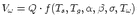 | (D.2) |
Q is the instrument static magnification. The amplitude characteristic f depends on the
natural periods of pendulum (Ts) and galvanometer (Tg), the damping constants of pendulum
( ) and galvanometer (
 ), the coupling coefficient () and the ground motion period T.
Following Hagiwara (1958) f, can be expressed as
), the coupling coefficient () and the ground motion period T.
Following Hagiwara (1958) f, can be expressed as
![u
f = V~ -----------------------4----------------3--
[1 - {a + 4abb}u2 + un2-]2 + [- 2cu + 2d un-]2](main104x.gif) | (D.3) |
where

The magnification V of the second group is (Galitzin, 1914):
 | (D.4) |
where T = Tg = Ts, l is the length of the pendulum, A1 the distance between the
galvanometer’s mirror and recording drum, k the transfer factor describing the galvanometer’s
sensitivity. For both types the measured amplitude A after removing the gain V , is true
ground displacement (in m).
_______________________________________________________________________________________
Bibliography
Abercrombie, R. E., 1994. Regional bias in estimates of earthquake MS due to
surface-wave path effects, Bull. Seism. Soc. Am., 84, 377-382.
Aki, K. & Richards, P. G., 2002. Quantitative seismology, University Science Book,
Sausalito, California.
Allegretti, I., Herak, D., Herak, M., & Duda, S. J., 2000. Consistency of magnitudes
of the largest earthquakes of the first half of the 20th century determined on the basis
of Göttingen and Zagreb seismograms, Studia geoph. et geod, 44, 13-25.
Ambraseys, N., 2003. Reappraisal of magnitude of 20th century earthquakes in
Switzerland, J. Earthq. Eng., 2, 149-191.
Ambraseys, N. & Douglas, J., 2000. Reappraisal of surface wave magnitudes in the
Eastern Mediterranean region and the Middle East, Geophys. J. Int., 141, 357-373.
Ambraseys, N. & Free, M., 1997. Surface wave magnitude calibration for European
region earthquakes, J. Earthq. Eng., 1, 1-22.
Arvidsson, R. & Ekstrom, G., 1998. Global CMT Analysis of moderate earthquakes,
Mw > 4.5, using intermediate-period surface waves, Bull. Seism. Soc. Am., 88,
1003-1013.
Baer, M., Deichmann, N., Braunmiller, J., Bernardi, F., Cornou, C., Fäh, D., Giardini,
D., Huber, S., Kästli, P., Kind, F., Kradolfer, U., Mai, M., Maraini, S., Oprsal, I., Schler,
T., Schorlemmer, D., Sellami, S., Steimen, S., Wiemer, S., Wössner, J., & Wyss, A.,
2003. Earthquakes in Switzerland and surrounding regions during 2002, Eclogae Geol.
Helv, 96, 313-324.
Bernardi, F., Braunmiller, J., Kradolfer, U., & Giardini, D., 2004. Automatic regional
moment tensor inversion in the European-Mediterranean region, Geophys. J. Int., 156,
1-14.
Bono, A., Simoni, B. D., Megna, A., Nardi, A., & Palombo, B., 2002. SISMOS project:
recovering and reprocessing of historical seismic data, ESC XXVIII general assembly,
Genova.
Boschi, L., Ekstrm, G., & Kustowski, B., 2004. Multiple resolution surface wave
tomography: the Mediterranean basin, Geophys. J. Int., 157, 293-304.
Bossu, R., Mazet-Roux, G., Tome, M., Carreno, E., Guilbert, J., Menechal, Y.,
Schindele, F., & di Giovambattista, R., 2002. EMSC early warning system and real
time seismicity, EMSC Newsletter, 18, 2-5.
Braunmiller, J., 1998. Seismotectonics of the Explorer Region and of the Blanco
Transform Fault Zone, Ph.D. thesis, Oregon State University.
Braunmiller, J., 2001. An European-Mediterranean regional moment tensor catalog -
year 2000, EOS, Trans., (82), Fall Meet. Suppl., Abstract S11B-0570.
Braunmiller, J., 2002. Moment tensor solutions of stronger earthquakes in Germany
with GRSN data, in Ten years of German regional seismic network (GRSN), pp.
227-235, Deutsche Forschungsgemeinschaft.
Braunmiller, J., Náb lek, J., Leitner, B., & Qamar, A., 1995. The 1993 Klamath
Falls, Oregon earthquake sequence: source mechanisms from regional data, Geophys.
Res. Lett., 22, 105-108.
lek, J., Leitner, B., & Qamar, A., 1995. The 1993 Klamath
Falls, Oregon earthquake sequence: source mechanisms from regional data, Geophys.
Res. Lett., 22, 105-108.
Braunmiller, J., Kradolfer, U., Baer, M., & Giardini, D., 2000. Regional moment-tensor
inversion in the European-Mediterranean area, Orfeus Newsletter, 2, 5.
Braunmiller, J., Kradolfer, U., Baer, M., & Giardini, D., 2002. Regional moment tensor
determination in the European-Mediterranean region - initial results, Tectonophysics,
356, 5-22.
Braunmiller, J., Deichmann, N., Giardini, D., & Wiemer, S., 2004. Homogeneous
moment magnitude calibration in Switzerland, accepted by Bull. Seism. Soc. Am..
Cotte, N. & Laske, G., 2002. Testing group velocitiy maps for Eurasia, Geophys. J.
Int., 150, 639-650.
Dahlen, F. A. & Tromp, J., 1998. Theoretical global seismology, Princeton University
Press, Priceton, New Jersey.
Davis, S. D. & Fröhlich, C., 1995. A comparison of moment tensor solutions in the
Harvard CMT and USGS catalogs, EOS, 76, F381.
Deichmann, N., 1992. Structural and rheological implications of lower-crustal
earthquakes below northern Switzerland, Phys. Earth planet. Int., 69, 270-280.
Deichmann, N., Baer, M., Braunmiller, J., Ballarin, D., Bay, F., Bernardi, F., Delouis,
B., Fäh, D., Gerstenberger, M., Giardini, D., Huber, S., Kradolfer, U., Maraini, S.,
Oprsal, I., Schibler, R., Schler, T., Sellami, S., Steimen, S., Wiemer, S., Wössner, J.,
& Wyss, A., 2002. Earthquakes in Switzerland and surrounding regions during 2001,
Eclogae Geol. Helv, 95, 249-261.
Dreger, D. S. & Helmberger, D. V., 1993. Determination of source parameters at
regional distances with three-component sparse network data, J. geophys. Res., 98,
8107-8125.
Dreger, D. S., Ritsema, J., & Pasyanos, M., 1995. Broadband analysis of the 21
September, 1993, Klamath Falls earthquake sequence, Geophys. Res. Lett., 105,
997-1000.
Dziewonski, A. M. & Anderson, D. L., 1981. Preliminary reference Earth model,
Phys. Earth planet. Int., 25, 297-356.
Dziewonski, A. M. & Woodhouse, J. H., 1983. An experiment in systematic study
of global seismicity: centroid-moment tensor solutions for 201 moderate and large
earthquakes of 1981, J. geophys. Res., 88, 3247-3271.
Dziewonski, A. M., Chou, T.-A., & Woodhouse, J. H., 1981. Determination of
earthquake source parameters from waveform data for studies of global and regional
seismicity, J. geophys. Res., 86, 2825-2852.
Ekström, G., 1987. A broad band method of earthquake analysis, Ph.D. thesis, Harvard
University, Cambridge, MA.
Ekström, G. & Dziewonski, M., 1988. Evidence of bias in estimations of earthquake
size, Nature, 332, 319-323.
Evernden, J. F., 1971. Variation of Rayleigh-wave amplitude with distance, Bull.
Seism. Soc. Am., 61, 231-240.
Fäh, D., Giardini, D., Bay, F., Bernardi, F., Braunmiller, J., Deichmann, N., Furrer,
M., Gantner, L., Gisler, M., Jimenez, D. I. M., Kästli, P., Koglin, R., Masciadri, V.,
Rutz, M., Scheidegger, C., Schibler, R., Schorlemmer, D., Schwarz-Zanetti, G., Steimen,
S., Sellami, S., Wiemer, S., & Wössner, J., 2003. Earthquake Catalog Of Switzerland
(ECOS) and the related macroseismic database, Eclogae geol. Helv., 96, 219-236.
Fröhlich, C., 1994. Earthquakes with non-double-couple mechanisms, Science, 264,
804-809.
Fröhlich, C., Millard, F. C., Massel, C., & Mann, P., 1997. Constraints on Macquarie
tectonics provided by Harvard focal mechanisms and teleseismic earthquake locations,
J. geophys. Res., 102, 5029-5041.
Galitzin, F. B., 1914. Vorlesungen über Seismometrie, B.G. Teuner.
Giardini, D., 1992. Moment tensor inversion from MEDNET data (1) large worldwide
earthquakes of 1990, Geophys. Res. Lett., 19, 713-716.
Giardini, D., Boschi, E., & Palombo, B., 1993a. Moment tensor inversion from
MEDNET data (2) regional earthquakes of the Mediterranean, Geophys. Res. Lett., 20,
273-276.
Giardini, D., Palombo, B., & Boschi, E., 1993b. The determination of earthquake size
and source geometry in the Mediterranean Sea, in: Recent evolution and seismicity of
the Mediterranean area, pp. 213-238, Kluwer.
Gutenberg, B., 1945. Amplitudes of Rayleigh-waves and magnitude of shallow
earthquakes, Bull. Seism. Soc. Am., 35, 3-12.
Hagiwara, T., 1958. A note on the theory of the electromagnetic seismograph, Bull.
Earth. Res. Inst., 36, 139-164.
Hanks, T. C. & Kanamori, H., 1979. A moment magnitude scale, J. geophys. Res.,
84, 2348-2350.
Helffrich, G. R., 1997. How good are routinely determined focal mechanisms?
Empirical statistics based on a comparison of Harvard, USGS and ERI moment tensors,
Geophys. J. Int., 131, 741-750.
Henry, C., Woodhouse, J. H., & Das, S., 2002. Stability of earthquake moment tensor
inversions: effect of the double-couple constraint, Tectonophysics, 356, 115-124.
Herak, M. & Herak, D., 1993. Distance dependence of MS and calibrating function
for 20 second Rayleigh waves, Bull. Seism. Soc. Am., 83, 1881-1892.
Herak, M., Allegretti, I., Herak, D., & Duda, S. J., 1996. Calibration of the Wiechert
seismograph relative to a reference seismometer, Geofisika, 13, 31-59.
IASPEI, 1967. Recommendations of the comittee on magnitudes, Comptes Rendus,
15, 65.
Jackson, J. A. & McKenzie, D., 1988. The relationship between plate motions and
seismic moment tensor, and the rates of active deformation in the Mediterranean and
Middle East, Geophys. J., 93, 45-73.
Jenny, S., Goes, S., Giardini, D., & Kahle, H.-G., 2004. Earthquake recurrence
parameters from seismic and geodetic strain rates in the eastern Mediterranean,
Geophys. J. Int., 157, doi:10.1111/j.1365-246X.2004.02261.x.
Jost, M. L. & Herrmann, R. B., 1989. A student’s guide and review to moment
tesnsors, Seism. Res. Lett., 60, 37-57.
Kanamori, H., 1977. The energy release in great earthquakes, J. geophys. Res., 82,
2981-2987.
Kanamori, H. & Anderson, D. L., 1975. Theoretical basis of some empirical relations
in seismology, Bull. Seism. Soc. Am., 65, 1073-1095.
Kárník, V., Kondorskaya, N., Riznitchenko, J., Savarensky, E., Soloviev, S., Shebalin,
N., Van k, N., & Zátopek, A., 1962. Standardisation of the earthquake magnitude
scale, Studia Geophys. Geodet., 6, 42-47.
k, N., & Zátopek, A., 1962. Standardisation of the earthquake magnitude
scale, Studia Geophys. Geodet., 6, 42-47.
Kastrup, U., Zoback, M. L., Deichmann, N., Evans, K. F., Giardini, D., &
Michael, A. J., 2004. Stress field variations in the Swiss Alps and northern Alpine
foreland derived from inversion of fault plane solutions, J. geophys. Res., B01402,
doi:10.1029/2003JB002550.
Kawakatsu, H., 1995. Automated near-realtime CMT inversion, Geophys. Res. Lett.,
22, 2569-2572.
Kennett, B. & Engdahl, E., 1991. Traveltimes for global earthquake location and phase
identification, Geophys. J. Int., 105, 429-465.
Knopoff, L. & Randall, M. J., 1970. The compensated linear-vector dipole: A possible
mechanism for deep earthquakes, J. geophys. Res., 75, 4957-4963.
Komatitsch, D. & Tromp, J., 2002. TSpectral-element simulations of global seismic
wave propagation - II. Three-dimensional models, oceans, rotation and self-gravitation,
Geophys. J. Int., 150, 303-318.
Kowalle,
G. & Thürmer, C., 1991. Magnitudenbestimmung für die Wiechert-Seismogramme der
Station Potsdam, Zentralinstitut für Physik der Erde, Potsdam.
Kradolfer, U., 1996. AutoDRM - the first five years, Seis. Res. Lett., 67, 30-33.
Kubo, A., Fukuyama, E., & Nonomura, K., 2002. NIED seismic moment tensor
catalogue for regional earthquakes around Japan: quality test and application,
Tectonophysics, 356, 23-48.
Kuge, K. & Kawakatsu, H., 1993. Significance of non-double couple components of
deep and intermediate-depth earthquakes: implications from moment tensor inversion
of long-period seismic waves, Phys. Earth planet. Int., 75, 243-266.
Kuge, K. & Lay, T., 1994. Data-dependent non-double-couple components of shallow
earthquake source mechanisms: Effects of waveform inversion instability, Geophys. Res.
Lett., 21, 9-12.
Kunze, T., 1982. Seismotektonische Bewegungen im Alpenbereich, Ph.D. thesis,
Universität Stuttgart.
Larson, E. W. & Ekström, G., 2001. Global models of surface wave group velocity,
Pure and Applied Geophysics, 158, 1377-1399.
Mainka, C., 1923. Physik der Erdbebenwellen, Verlag Gebrüder Borntraeger, Berlin.
Marone, F., van der Meijde, M., van der Lee, S., & Giardini, D., 2003. Joint inversion
of local, regional and teleseismic data for crustal thickness in the Eurasia-Africa plate
boundary region, Geophys. J. Int., 154, 499-514.
Marone, F., van der Lee, S., & Giardini, D., 2004. Shallow anisotropy in
the Mediterranean mantle from surface waves, Geophys. Res. Lett., 31, L06624,
doi:10.1029/2003GL018948.
Maset-Roux, G. & Bossu, R., 2004. Report on emsc operational activities, Tech. rep.,
European-Mediterranean Seismological Centre.
Náb lek, J. & Xia, G., 1995. Moment-tensor analysis using regional data: application
to the 25 March, 1993, Scotts Mills, Oregon, earthquake, Geophys. Res. Lett., 22, 13-16.
lek, J. & Xia, G., 1995. Moment-tensor analysis using regional data: application
to the 25 March, 1993, Scotts Mills, Oregon, earthquake, Geophys. Res. Lett., 22, 13-16.
Panza, G. F., Duda, S. J., Cernobori, L., & Herak, M., 1989. Gutenberg’s
surface-wave magnitude calibrating function: theoretical basis from synthetic
seismograms, Tectonophysics, 166, 35-43.
Pasyanos, M. E., Dreger, D. S., & Romanowicz, B., 1996. Toward real-time estimation
of regional moment tensors, Bull. Seism. Soc. Am., 86, 1255-1269.
Pasyanos, M. E., Walter, W. R., & Hazler, S. E., 2001. A surface wave dispersion
study of the Middle East and North Africa for monitoring the comprehensive
Nuclear-Test-Ban Treaty, Pure and Applied Geophysics, 158, 1445-1474.
Patton, H. & Aki, K., 1979. Bias in the estimate of seismic moment tensor by the
linear inversion method, Geophys. J. R. astr. Soc., 59, 479-495.
Peterson, J., 1993. Observations and modeling of seismic background noise., U.S.
Departement of Interior, Geological Survey, pp. Open-File Report 93-322.
Pondrelli, S., Morelli, A., Ekström, G., Mazza, S., Boschi, E., & Dziewonski, A. M.,
2002. European-Mediterranean regional centroid-moment tensors: 1997-2000, Phys.
Earth planet. Int., 130, 71-101.
Rezapour, M. & Pearce, R. G., 1998. Bias in surface-wave magnitude MS due to
inadequate distance corrections, Bull. Seism. Soc. Am., 88, 43-61.
Ritsema, J. & Lay, T., 1993. Rapid source mechanism determination of large (Mw >
4.5) earthquakes in western United States, Geophys. Res. Lett., 20, 1611-1614.
Ritter, J. R. R., 2001. On the recording characteristics of the original Wiechert
seismographs at Göttingen (Germany), Journal of Seismology, 6, 477-486.
Romanowicz, B., Dreger, D., Pasyanos, M., & Uhrhammer, R., 1993. Monitoring strain
release in central and northern California using broadband data, Geophys. Res. Lett.,
20, 1643-1646.
Sicilia, D., 1999. Towards regional moment tensor determination: the moment tensor
of the 1994 mb = 4.8 event near the Balearic Islands and its uncertainties, Diploma
thesis, ETH Zürich.
 ílený, J. & Vavry
 uk, V., 2002. Can unbiased source be retrieved from anisotropic
waveforms by using an isotropic model of the medium?, Tectonophysics, 356, 125-138.
uk, V., 2002. Can unbiased source be retrieved from anisotropic
waveforms by using an isotropic model of the medium?, Tectonophysics, 356, 125-138.
Sipkin, S. A., 1982. Estimation of earthquake source parameters by the inversion of
waveform data: synthetic waveforms, Phys. Earth planet. Int., 30, 242-259.
Sipkin, S. A., 1986. Estimation of earthquake source parameters by the inversion of
waveform data: global seismicity, 1981-1983, Bull. Seism. Soc. Am., 76, 1515-1541.
Soloviev, S. L., 1955. O klassifikatsii zemletrasenii po velichine ikh energii, Trudi
Geofiz. Inst. Akad. Nauk SSSR, 30, 3-31.
Stahel, W. A., 1995. Statistische Datenanalyse, Friedr. Vieweg & Sohn
Verlagsgesellschaft mbH, Braunschweig/Wiesbaden.
Stich, D., Ammon, C. J., & Morales, J., 2003. Moment tensor solutions for small and
moderate earthquakes in the Ibero-Maghreb region, J. geophys. Res., 108(B3), 2148,
doi:10.1029/2002JB002057.
Thio, H.-K. & Kanamori, H., 1995. Moment tensor inversion for local earthquakes
using surface waves recorded at TERRAscope, Bull. Seism. Soc. Am., 85, 1021-1038.
van der Lee, S., 1998. Observation and origin of Rayleigh-wave amplitude anomalies,
Geophys. J. Int., 135, 691-699.
van Eck, T., Dost, B., & Hanka, W., 2001. European scale real-time waveform data
exchange, EMSC Newsletter, 17, 11.
van Eck, T., Trabant, C., Dost, B., Hanka, W., & Giardini, D., 2004. Setting up a
virtual Broadband seismograph network acorss Europe, EOS, 85, 125,129.
Van k, N., Zátopek, A., Kárník, V., Kondorskaya, N., Riznitchenko, J., Savarensky,
E., Soloviev, S., & Shebalin, N., 1962. Standardisation of magnitude scales, Bull. Acad.
Sci. USSR, Geophys. Ser., 2, 108-111.
k, N., Zátopek, A., Kárník, V., Kondorskaya, N., Riznitchenko, J., Savarensky,
E., Soloviev, S., & Shebalin, N., 1962. Standardisation of magnitude scales, Bull. Acad.
Sci. USSR, Geophys. Ser., 2, 108-111.
von Seggern, D., 1977. Amplitude-distance for 20-second Rayleigh waves, Bull. Seism.
Soc. Am., 67, 405-411.
Wessel, P. & Smith, W. H. F., 1995. New version of the generic mapping tool released,
Trans. Am. Geophys. Union, p. 329.
Wiechert, E., 1903. Theorie der automatischen Seismographen, Weidmannsche
Buchhandlung.
Willmore, P. L., 1979. Manual of seismological observatory practice, World Data
Center A for Solid Earth Geophysics.
Woodhouse, J. H., 1988. The calculation of eigenfrequencies and eigenfunctions of the
free oscillations of the Earth and the Sun, in: Seismological algorithms, pp. 321-370,
Academic Press.
Zhang, J. & Lay, T., 1990. Effects of centroid location on determination of earthquake
mechanisms using long-period surface waves, Bull. Seism. Soc. Am., 80, 1205-1231.
Curriculum Vitae
Personal
Date of birth | 30 June 1973 |
Place of birth | Lugano, Switzerland |
Citizen of | Stabio, Switzerland |
| |
Education
2000-2004 | PhD. student at institute of Geophysics at the Swiss Federal
Institute of Technology in Zürich, Switzerland |
1994-2000 | Study of Earth Sciences with major in Geophysics at the Swiss
Federal Institute of Technology in Zürich, Switzerland |
1988-1992 | High School in Mendrisio, Switzerland |
| |